american
Parameter estimation for power-law distributions
by maximum likelihood methods
Abstract
Distributions following a power-law are an ubiquitous phenomenon. Methods for determining the exponent of a power-law tail by graphical means are often used in practice but are intrinsically unreliable. Maximum likelihood estimators for the exponent are a mathematically sound alternative to graphical methods.
pacs
02.50.Tt, 89.75.-k1 Introduction
The distribution of a discrete random variable is referred to as a distribution with a power-law tail if it falls as
| (1) |
for and . Power-laws are ubiquitous distributions that can be found in many systems from different disciplines, see [1, 2] and references therein for some examples.
Experimental data of quantities that follow a power-law are usually very noisy; and therefore obtaining reliable estimates for the exponent is notoriously difficult. Estimates that are based on graphical methods are certainly used most often in practice. But simple graphical methods are intrinsically unreliable and not able to establish a reliable estimate of the exponent .
For that reason, the authors of [3] introduced an alternative approach based on a maximum likelihood estimator for the exponent . Unfortunately the authors concentrate on a rather idealized type of power-law distributions, namely
| (2) |
with , where the normalization constant is given by the Hurwitz--function which is defined for and by
| (3) |
The distribution (2) is characterized by one parameter only, and therefore all properties of this distribution (e. g. its mean) are determined solely by the exponent . In many applications the power-law (2) is too restrictive.
If one states that a quantity follows a power-law, then this means usually that the tail () of the distribution falls proportionally to . Probabilities for may differ from the power-law and admit the possibility to tune the mean or other characteristics independently of . In some situations probabilities may differ from a power-law for as well, e. g. the distribution may have an exponential cut-off.
Therefore, I will generalize the maximum likelihood approach introduced in [3] to distributions that follow a power-law within a certain range but differ from a power-law outside this range in an arbitrary way. Furthermore, I will give some statements about the large sample properties of the estimate of the power-law exponent and present a numerical procedure to identify the power-law regime of the distribution . But first, let us see what is wrong with popular graphical methods.
2 Trouble with graphical methods
All graphical methods for estimating power-law exponents are based on a linear least squares fit of some empirical data points , ,…, to the function
| (4) |
The linear least squares fit minimizes the residual
| (5) |
Estimates and of the parameters and are given by [4]
| (6) | ||||
| and | ||||
| (7) | ||||
The ansatz for the residual (5) and derivation of (6) and (7) are based on several assumptions regarding the data points . It is assumed that there are no statistical uncertainties in , but may contain some statistical error. The errors in different are independent identically distributed random variables with mean zero. In particular the standard deviation of the error is independent of . For various graphical methods for the estimation of the exponent of a power-law distribution these conditions are not met, leading to the poor performance of these methods.
fit on the distribution
fit on the cumulative distribution
no binning
a) 
b) 
logarithmic binning
c) 
d) 
To illustrate the failure of graphical methods by a computer experiment random numbers had been drawn from distribution (2) with and an estimate for the exponent was determined by various graphical methods. The estimator is a random variable and its distribution depends on the method that has been used to obtain the estimate. Important measures of the quality of an estimator are its mean and its standard deviation. If the mean of the estimator equals the true exponent then the estimator is unbiased and estimators with a distribution that is concentrated around are desirable. For each graphical method a histogram of the distribution of the estimator was calculated to rate the quality of the estimator by repeating the numerical experiment 500 times.
The most straight forward (and most unreliable) graphical approach is based on a plot of the empirical probability distribution on a double-logarithmic scale. Introducing the indicator function , which is one if the statement in the brackets is true and else zero, the empirical probability distribution is given by
| (8) |
An estimate for the power-law exponent is established by a least squares fit to
| (9) |
equals the estimate (7) for the slope, see Figure 1 a. Because the lack of data points in the tail of the empirical distribution this procedure underestimates systematically the exponent , see Table 1.
| mean | standard deviation | |
|---|---|---|
| method | estimate | of estimate |
| fit on empirical distribution | 1.597 | 0.167 |
| fit on cumulative empirical distribution | 2.395 | 0.304 |
| fit on empirical distribution with logarithmic binning00 0 In [3] a similar experiment is reported. For a fit of the logarithmically binned empirical probability distribution the authors find a systematical bias of 29 %. I cannot reconstruct such a strong bias, instead I get a bias of 5 % only. Probably the quality of this method depends on the details of the binning procedure. | 2.397 | 0.080 |
| fit on cumulative empirical distribution with logarithmic binning | 2.544 | 0.127 |
| maximum likelihood | 2.500 | 0.016 |
There are two ways to deal with the sparseness in the tail of the empirical distribution, logarithmic binning and considering the empirical cumulative distribution instead of . The cumulative probability distribution of (2) is defined by
| (10) |
If has a power-law tail with exponent then follows approximately a power-law with exponent because for the distribution can be approximated by
| (11) |
The empirical cumulative probability distribution is given by
| (12) |
It is less sensitive to the noise in the tail of the distribution and therefore a fit of
| (13) |
to a straight line gives much better estimates for the exponent, see Figure 1 b. But there is still a small bias to too small values and the distribution of this estimate is rather broad, see Table 1.
Logarithmic binning reduces the noise in the tail of the empirical distributions and by merging data points into groups. By introducing the logarithmically scaled boundaries
| (14) |
(The function rounds to the nearest integer.) a linear least squares fit is performed to
| (15) | ||||
| or | ||||
| (16) | ||||
respectively. As a consequence of the binning the width of the distribution of the estimate of the power-law exponent is reduced, see Figure 1 c, 1 d and Table 1. According to the numerical experiments a fit of the logarithmically binned cumulative distribution gives the best results among graphical methods. It shows the smallest systematic bias.
All the methods that have been considered so far have a common weakness. In the deviation of (6) and (7) it was assumed that the standard deviation of the distribution of the error in is the same for all data points . But this is obviously not the case. For fixed the empirical distribution is a random variable with mean and standard deviation . For the corresponding data on a logarithmic scale the standard deviation is approximately given by the quotient
| (17) |
A power-law distribution is a monotonically decreasing function and therefore (17) is an increasing function of . Because the variation of the statistical error is not taken into account, the distribution of the estimate is very broad.
Methods that deal with the cumulative distribution have an additional weakness. Cumulation has the side-effect that the statistical errors in are not independent any more, which violates another assumption of the deviation of (6) and (7).
To sum up, estimates of exponents of power-law distributions based on a linear least squares fit are intrinsically inaccurate and lack a sound mathematical justification.
3 Maximum likelihood estimators
Maximum likelihood estimators offer a solid alternative to graphical methods. Let denote a single parameter probability distribution. The maximum likelihood estimator for the unknown parameter based on a sample of size is given by
| (18) |
where
| (19) |
denotes the likelihood function. In the limit of asymptotically large samples and under some regularity conditions maximum likelihood estimators share some desirable features [5, 6].
- •
The estimator exists and is unique.
- •
The estimator is consistent, that means for every
(20) where denotes the probability that the difference is less than .
- •
The estimator is asymptotically normal with mean and variance
(21) where indicates the expectation value of the quantity in the brackets.
- •
Maximum likelihood estimators have asymptotically minimal variance among all asymptotically unbiased estimators. One says, they are asymptotically efficient.
4 Maximum likelihood estimators for genuine power-laws
The most general discrete genuine power-law distribution has a lower as well as an upper bound and is given by
| (22) |
for with . Where the non-standard notation
| (23) |
has been introduced. If the upper bound is missing the distribution
| (24) |
has to be considered for with . The distributions (22) and (24) are generalizations of (2) and will be useful for the analysis of more general distributions that show a power-law behavior only in a certain range but have an arbitrary profile outside the power-law regime. This kind of distributions will be considered in section 5.
The maximum likelihood estimator for the parameter of the distribution (22) follows from (18) and is given by
| (25) |
or equivalently by the implicit equation
| (26) |
which has to be solved numerically. The prime denotes the derivative with respect to . The asymptotic variance of this estimator follows from (21) and equals
| (27) |
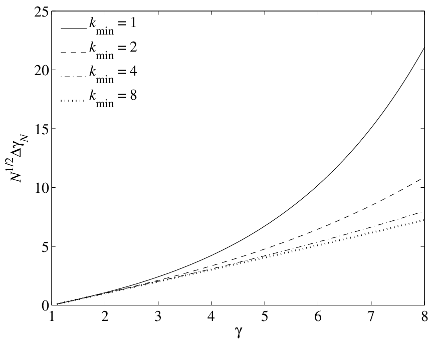
In the limit equations (25), (26), and (27) give the maximum likelihood estimator and the asymptotic variance of this estimator for power-law distributions lacking an upper cut-off (24). A graphical representation of the standard deviation (27) in the limit is given in Figure 2. For each fixed the quantity grows faster than linear with . Therefore the larger the exponent the larger the sample size that is necessary to get an estimate within a given error bound.

If the maximum likelihood method is applied (assuming a distribution (24)) to the same data as in section 2, numerical experiments show that the estimates for the exponent are much more precise. The estimate has no identifiable systematic bias, the standard deviation of the distribution of the estimate is smaller by an order of magnitude compared to graphical methods, see Table 1 and Figure 3.
5 Maximum likelihood method for general power-law distributions
The maximum likelihood procedure outlined in section 4 can be generalized further to distributions that are no pure power-laws (22) or (24) but follow a power-law within a certain finite range or follow a power-law in the whole tail of the distribution and have an arbitrary profile outside the power-law regime. The popurse of this section is to establish methods for identifying the power-law regime and for estimating the exponent of the power-law regime without making special assumptions about the profile of the probability distribution beyond the power-law regime.
The main problem for a generalization of the maximum likelihood approach is that there might be no good hypothesis for the profile of the probability distribution beyond the power-law regime. To overcome this difficulty the empirical data set is restricted to a window . (The following discussion covers the case of a power-law tail distributions as well by setting .) Assuming that has a power-law profile for then the probability distribution of the restricted data set is given by (22) with and (or by (24) with ) and some unknown exponent . This allows to estimate the power-law exponent by the application of the maximum likelihood method on the restricted data set of size as presented in section 4 without making a hypothesis about the profile of the probability distribution beyond the power-law regime.
In order to apply the maximum likelihood method one has to determine the cut-off points and first. Here it has to be taken into account that if the window is chosen too large the estimate is systematically biased, but on the other hand if it is too small the statistical error is larger than necessary. In some cases one can make conservative estimates for and by plotting the empirical probability distribution (8) on a double-logarithmic scale. An appropriate window can also be found by determining estimates as a function of the window and a -test.
Assuming the empirical data is drawn from a distribution with a power-law tail (no upper cut-off) the lower cut-off point can be determined in the following systematic way. By varying the parameter the maximum likelihood approach gives a sequence of estimates . If is very large the estimate will be quite inaccurate because only a tiny fraction of the experimental data is taken into account; but the smaller the cut-off the more accurate the estimate of the exponent. If approaches the point from above (but is still above) where the probability distribution starts do differ from a power-law will give a very precise estimate for the exponent . On the other hand, if is too small the hypothesis that the (restricted) empirical data is drawn from a power-law distribution is violated which causes a significant change of the estimate of the power-law exponent.
If the empirical data is drawn from a distribution having both a lower crossover point as well as an upper crossover point a sequence of estimates is determined by restricting the data to a sliding window with . As long as the window lies completely within the power-law regime the maximum likelihood estimate obtained from the restricted data set will give a reliable estimate of the power-law exponent. If the window lies at least partly outside the power-law regime the estimate is systematically biased.

To illustrate the procedures outlined above I generated two data sets from two distributions having a power-law regime. The first data set of samples was drawn from a distribution with a power-law tail which is given by
| (28) |
Plotting the sequence of estimates against the parameter reveals the exponent as wells as the crossover point very clearly, see Figure 4. The second data set of samples was drawn from a distribution with two crossover points, viz.
| (29) |
Figure 5 shows the sequence of estimates that had been determined from restricted data sets of samples within the sliding window . This sequence exhibits a broad plateau that corresponds to the power-law exponent . If the window does not lie completely inside the power-law regime the estimate deviates systematically from the known exponent.

Apart from a visual inspection of the plot the crossover point(s) to the power-law regime can be determined by means of a -test. To apply a -test the data set has to be divided into some bins and the following binning turned out to be appropriate: The data is partitioned into a small number , say , of bins. In the case of a distribution with a power-law tail this means each bin collects items such that
| (30) | ||||||
| (31) | ||||||
| and finally | ||||||
| (32) | ||||||
where denotes the probability that a data point falls into bin under the assumption that the (restricted) data follows the power-law (24) with and the exponent . For distributions with a finite power-law regime the binning procedure can be carried out in a similar way. In this case the summation index in (32) is bounded by and the probability has to be considered instead of .
The test statistic of the -test is given by
| (33) |
If the to restricted data is given by the power-law (22) or (24) with , , and the exponent then the statistic follows asymptotically a -distribution with degrees of freedom, which is given by
| (34) |
Let be the -quantile of the distribution (34). The hypothesis that the restricted data is given by the power-law (22) or (24), respectively, with , , and the exponent is accepted with the error probability if . If the window lies not completely within the power-law regime this hypothesis will be rejected by the -test and one can detect the upper crossover point as well as the lower crossover point (where the power-law loses its validity) in a reliable way, see Figure 4 and Figure 5.
6 Computational remarks
The normalizing factors of the probability distributions (22) and (24) are given by the Hurwitz--function. This function is less common than other special functions and may not be available in the reader’s favorite statistical software package but the GNU Scientific Library [7] offers an open source implementation of this function. A direct calculation of the Hurwitz--function by truncating the sum (3) gives unsatisfactory results.
The maximum likelihood estimator of the exponent can be computed numerically either by solving (25) or (26). Equation (25) has the advantage that it can be solved without calculating derivatives of the Hurwitz--function [8], whereas the solution of (26) involves its first derivative (e. g. bisection method) or even higher derivatives (e. g. Newton-Raphson method). An explicit implementation of these derivatives is often not available but may be calculated numerically.
7 Conclusion
Methods based on a least squares fit are not suited to establish estimates for power-law distribution exponents because least squares fits rely on assumptions about the data set that are not fulfilled by empirical data from power-law distributions. In this paper maximum likelihood estimators have been introduced as a reliable alternative to graphical methods. These estimators are asymptotically efficient and can be applied to data from a wide class of distributions having a power-law regime. The crossover points that separate the power-law regime from the rest of the distribution can be determined by a procedure based on a -test.
Finally I would like to mention that the idea to plot a sequence of estimates as shown in Figure 4 is related to so-called Hill plots [9, 10]. The Hill estimator is a maximum likelihood estimator for the inverse of the exponent of the continuous Pareto distribution , see [10] for a detailed discussion.
Acknowledgements.
Work sponsored by the European Community’s FP6 Information Society Technologies programme under contract IST-001935, EVERGROW.References
- [1] M.E.J. Newman, Contemporary Physics 46(5), 323 (2005)
- [2] E.F. Keller, BioEssays 27(10), 1060 (2005)
- [3] M.L. Goldstein, S.A. Morris, G.G. Yen, The European Physical Journal B 41(2), 255 (2004)
- [4] F. Ramsey, D. Schafer, The Statistical Sleuth: A Course in Methods of Data Analysis, 2nd edn. (Duxbury Press, Pacific Grove, CA, 2002)
- [5] L.J. Bain, M. Engelhardt, Introduction to Probability and Mathematical Statistics, Duxbury Classic Series, 2nd edn. (Duxbury Press, 2000)
- [6] Y. Pawitan, In all likelihood: statistical modelling and inference using likelihood, Oxford science publications (Oxford University Press, 2001)
- [7] GNU Scientific Library, http://www.gnu.org/software/gsl/
- [8] R.P. Brent, Algorithms for Minimization without Derivatives (Prentice-Hall, Englewood Cliffs, New Jersey, 1973)
- [9] B.M. Hill, Annals of Statistics 3(5), 1163 (1975)
- [10] H. Drees, L. de Haan, S. Resnick, Annals of Statistics 28(25), 254 (2000)