Parallelizing Quantum Circuits

Anne Broadbent Affiliation: Département d’informatique Affiliation: et de recherche opérationnelle Affiliation: Université de Montréal Email: broadbea@iro.umontreal.ca Elham Kashefi Affiliation: Christ Church College & Affiliation: Computing Laboratory Affiliation: University of Oxford Email: elham.kashefi@comlab.ox.ac.uk

April 12, 2007

Abstract

We present a novel automated technique for parallelizing quantum circuits via forward and backward translation to measurement-based quantum computing patterns and analyze the trade off in terms of depth and space complexity. As a result we distinguish a class of polynomial depth circuits that can be parallelized to logarithmic depth while adding only polynomial many auxiliary qubits. In particular, we provide for the first time a full characterization of patterns with flow of arbitrary depth, based on the notion of influencing paths and a simple rewriting system on the angles of the measurement. Our method leads to insightful knowledge for constructing parallel circuits and as applications, we demonstrate several constant and logarithmic depth circuits. Furthermore, we prove a logarithmic separation in terms of quantum depth between the quantum circuit model and the measurement-based model.

1 Introduction and summary of results

We present a construction for the parallelization of quantum circuits. Our method gives a formula that computes the exact decrease in depth that the construction can achieve. This yields precious insight for the construction of lower-depth quantum circuits.

The development of parallel quantum circuits seems almost essential if we wish to implement quantum algorithms in the near future with the available technology. Due to decoherence, qubits have a tendency to spontaneously change their state, hence we can only operate on them for a very short period of time. Parallel circuits could maximize the use of these fragile qubits. Note that to obtain parallelism in the quantum circuit model, we need the ability of interaction with further apart qubits. Different implementations might put physical limitations on how far we can apply this ability. However, in some recent proposals for quantum computing [1, 2, 3, 4, 5, 6, 7] due to the construction of the models, the far apart interaction between qubits have been successfully demonstrated.

As for theoretical motivation, the study of parallel quantum algorithms could lead to new results in complexity theory. For instance, one interesting open question is whether the class of decision problems solvable in polynomial time, ${\mathbf{P}}$ , is included in the class of decision problems solvable in polylogarithmic depth, ${\mathbf{NC}}$ . Let ${\mathbf{QNC}}$ be the class of decision problems solvable in polylogarithmic depth with a quantum computer, one can ask similarly whether ${\mathbf{P}}$ is included in ${\mathbf{QNC}}$ . Finally, Richard Jozsa conjectured that:

Jozsa Conjecture.[8] Any polynomial-time quantum algorithm can be implemented with only $O(\log(n))$ quantum layers interspersed with polynomial-time classical computations.

Previous results on parallel quantum circuits include the parallelization of circuits for the semi-classical quantum Fourier transform [9], approximate quantum Fourier transform [10], as well as for encoding and decoding quantum error-correcting codes [11]. These constructions usually require the use of auxiliary qubits. The depth complexity of quantum circuits has also been studied in [12, 13].

Our results on parallelizing quantum circuits (Theorem 8.7) are obtained using the recently proposed formalism of the measurement-based model for quantum computation (MBQC) [8, 14, 15, 16], an approach to quantum computing that uses measurement as its main ingredient. A computation in MBQC is usually referred to as a pattern and consists of a round of global operations (two-qubit gates) to create the required initial multi-qubit entanglement, followed by a sequence of classically controlled local operators (single qubit measurements and unitaries). A more formal definition is given later. We will work in particular within an algebraic framework for MBQC called the measurement calculus [17]. This novel framework is universal and equivalent in computational power to the quantum circuit model.¹¹ 1 In this paper whenever we mention a quantum circuit or a pattern we mean a uniform family of quantum circuits or patterns, where their descriptions are given by a classical Turing machine. Previous results on the parallelization in the MBQC include constant-depth patterns for Clifford unitaries [18] and diagonal unitaries [16].

The measurement calculus framework clearly distinguishes between the quantum and classical depths of a pattern. Informally speaking, the quantum depth of a pattern is the length of the longest sequence of dependent commands. The classical depth is the depth of the classical computation required for the evaluation of the dependency function of each dependent command. We consider two transformations that we can apply to patterns without changing their meaning (the underlying operator that they implement) while never increasing their depth (and possibly decreasing it): standardization (Theorem 4.1) and signal shifting (Theorem 5.1). Standardization is a rewriting system for MBQC patterns that pushes all the entanglement operators to the beginning of the computation, followed by a sequence of the single-qubit measurements and a final round of local unitaries. Signal shifting is another rewriting system that translates some of the quantum depth between measurement operators to classical depth between the final local unitaries and hence decreases the quantum depth.

We then develop a method to compute an upper bound on the quantum depth of a pattern. In order to do so, we use the notion of flow [19], a graph theoretical tool defined over the underlying geometry of the initial entanglement state of a pattern. We further define a construction called an influencing path, that allows us to characterize the dependency structure of the pattern. It is known that a particular set of measurements called Pauli measurements can be performed independently as the first layer of measurements [14]. Combining this fact about the angles of the measurement with influencing paths and the signal shifting procedure, we present an upper bound result on the quantum depth (Proposition 6.4). As for the classical depth, it is known to be at most logarithmic in the size of the pattern [8]. We give some tighter upper bounds based on the underlying geometry in Section 6.1.

Our ultimate goal is to decrease the depth of a given circuit, to this end we present an automated procedure for the translation of a circuit (with $g$ gates) to an MBQC pattern by adding only up to $g$ extra auxiliary qubits. Performing standardization and signal shifting over the obtained pattern might decrease the depth, and we then translate back the obtained low depth pattern to another circuit, equivalent to the original circuit but with lower quantum depth and more auxiliary qubits. This final translation is based on performing coherent measurements, and therefore the new circuit will have a depth equal to the combined quantum and classical depths of the pattern. Note that since classical computation is cheaper than quantum computation, one might consider MBQC as a favourable ultimate architecture for a quantum computer as it keeps the quantum and classical depth separate. However, this translation forward and backward to MBQC is interesting from the theoretical point of view as one can parallelize a circuit automatically and moreover due to the simplicity of the translation procedure the pattern depth characterization of Theorem 8.3 leads to a general parallelization result for circuits, Theorem 8.7.

As already noted, the depth of a pattern is due to the adaptive measurements and corrections: any given qubit has a fixed set of measurement outcomes that must be known before a measurement or a correction command can be performed at that qubit. This set of measurement dependencies is sometimes called the backward cone [18]. One way of interpreting our main result given by Theorem 8.3 is that we characterize the backward cone of any qubit; thus for patterns with flow, we are able to give a method to easily compute the depth. Moreover our characterization result is constructive and leads to a novel technique for constructing parallel patterns and parallel circuits.

In order to demonstrate the power of Theorems 8.3 and 8.7, we present some special cases: depth 2 patterns (Proposition 8.4) and depth 2 circuits (Proposition 8.8). Another application of our results is Proposition 8.9, where we show that any polynomial-size circuit with only Clifford gates can be parallelized to a logarithmic depth circuit, using a polynomial number of auxiliary qubits. Using the example of parity, we also show a logarithmic separation in terms of quantum depth between the circuit model and the MBQC. Finally, we show how our method can be used to parallelize a family of polynomial-depth circuits to equivalent logarithmic depth circuits.

The paper is organized as follows. In Section 2, we briefly review the MBQC in order to fix the relevant notation (a more thorough introduction to quantum computing and MBQC are available in appendices A and B). In Section 3, we define the notion of depth for a pattern in the MBQC, carefully distinguishing between the preparation, quantum and classical computation depths. In Section 4, we show that standardization decreases depth and in Section 5, we show that signal shifting also decreases depth. In Section 6, we give upper bounds on the depth of a pattern based on its geometry. In Section 7, we give a translation from the quantum circuit model to the measurement-based model and back. Our main results on characterization of depth for MBQC patterns and quantum circuits are given in Section 8, where we also present several applications.

2 Preliminaries

2.1 Quantum circuit model

Historically, Richard Feynman was one of the first to suggest that a computer based on the principles of quantum mechanics could efficiently simulate other quantum systems [20]. David Deutsch then developed the idea that the quantum computer could offer a computational advantage compared to the classical computer; he also defined the quantum Turing machine [21], before defining the quantum circuit model [22] to represent quantum computations (Deutsch refers to a quantum circuit as a quantum network). It is readily seen that the quantum circuit model is a generalization of the classical circuit model.

Any unitary operation $U$ can be approximated with a circuit $C$ , using gates in a fixed universal set of gates (see Appendix A or [23] for an introduction to quantum computing). The size of a circuit is the number of gates and its depth is the largest number of gates on any input-output path. Equivalently, the depth is the number of layers that are required for the parallel execution of the circuit, where a qubit can be involved in at most one interaction per layer. In this paper, we adopt the model according to which at any given timestep, a single qubit can be involved in at most one interaction. This differs from the concurrency viewpoint, according to which all interactions for commuting operations can be done simultaneously.

2.2 Measurement-based model

We give a brief introduction to the MBQC (a more detailed description is available in Appendix B or [8, 15, 16, 17]). Our notation follows that of [17].

Computations involve the following commands: 1-qubit preparations $N_{i}$ (prepares qubit $i$ in state ${|}+\rangle_{i}$ ), 2-qubit entanglement operators $E_{ij}:=\mathop{\wedge}\hskip-1.72218ptZ_{ij}$ (controlled- $Z$ operator), 1-qubit destructive measurements ${M}_{i}^{\alpha}$ , and 1-qubit Pauli corrections $X_{i}$ and $Z_{i}$ , where $i$ , $j$ represent the qubits on which each of these operations apply, and $\alpha\in[0,2\pi)$ . Measurement ${M}_{i}^{\alpha}$ is defined by orthogonal projections onto the state ${|}+_{\alpha}\rangle_{i}$ (with outcome $s_{i}=0$ ) and the state ${|}-_{\alpha}\rangle_{i}$ (with outcome $s_{i}=1$ ), where ${|}\pm_{\alpha}\rangle$ stands for $\frac{1}{\sqrt{2}}({|}0\rangle\pm e^{i\alpha}{|}1\rangle)$ . Measurement outcomes can be summed (modulo $2$ ) resulting in expressions of the form $s=\sum_{i\in I}s_{i}$ which are called signals.

Dependent corrections are written as $X_{i}^{s}$ and $Z_{i}^{s}$ , with $X_{i}^{0}=Z_{i}^{0}=I$ , $X_{i}^{1}=X_{i}$ , and $Z_{i}^{1}=Z_{i}$ , while dependent measurements are written as ${}_{t}[{M}_{i}^{\alpha}]^{s}$ with

\begin{array}[c]{lllllllllllllll}{}_{t}[{M}_{i}^{\alpha}]^{s}=M^{\alpha}_{i}X^{s}_{i}Z^{t}_{i}={M}_{i}^{(-1)^{s}\alpha+t\pi}\,.\end{array}

The right and left dependency of a measurement are called $X$ -dependency and $Z$ -dependency.

A pattern $\mathcal{P}$ is a finite sequence of commands acting on a finite set of qubits $V$ , for which $I\subset V$ and $O\subset V$ are input and output sets, respectively. Patterns are executed from right to left. We assume for the rest of the paper that all the non-input qubits are prepared and sometimes omit the preparation commands to be performed at these qubits.

By applying the following rewrite rules (1)–(4) of the measurement calculus [17], we find the standard form of a pattern, which is an ordering of the commands in the following order: preparation, entanglement, measurement and correction. Standardization is the procedure of applying the rewrite rules until no further rules are applicable.

$\displaystyle E_{ij}X_{i}^{s}$	$\displaystyle\Rightarrow$	$\displaystyle X_{i}^{s}Z_{j}^{s}E_{ij}$	(1)
$\displaystyle E_{ij}Z_{i}^{s}$	$\displaystyle\Rightarrow$	$\displaystyle Z_{i}^{s}E_{ij}$	(2)
$\displaystyle{}_{t}[{M}_{i}^{\alpha}]^{s}X_{i}^{r}$	$\displaystyle\Rightarrow$	$\displaystyle{}_{t}[{M}_{i}^{\alpha}]^{s+r}$	(3)
$\displaystyle{}_{t}[{M}_{i}^{\alpha}]^{s}Z_{i}^{r}$	$\displaystyle\Rightarrow$	$\displaystyle{}_{r+t}[{M}_{i}^{\alpha}]^{s}$	(4)

A pattern which is not in the standard form is called a wild pattern.

The signal shifting rules (5)–(8) tell us how to propagate $Z$ -dependencies; we refer to signal shifting as the procedure of applying the signal shifting rules until no further rules are applicable:

$\displaystyle{}_{t}[{M}_{i}^{\alpha}]^{s}$	$\displaystyle\Rightarrow$	$\displaystyle S_{i}^{t}\;[{M}_{i}^{\alpha}]^{s}$	(5)
$\displaystyle X_{j}^{s}S_{i}^{t}$	$\displaystyle\Rightarrow$	$\displaystyle S_{i}^{t}\;X_{j}^{s[(t+s_{i})/s_{i}]}$	(6)
$\displaystyle Z_{j}^{s}S_{i}^{t}$	$\displaystyle\Rightarrow$	$\displaystyle S_{i}^{t}\;Z_{j}^{s[(t+s_{i})/s_{i}]}$	(7)
$\displaystyle{}_{t}[{M}_{j}^{\alpha}]^{s}S_{i}^{r}$	$\displaystyle\Rightarrow$	$\displaystyle S_{i}^{r}\;{}_{t[(r+s_{i})/s_{i}]}[{M}_{j}^{\alpha}]^{s[(r+s_{i})/s_{i}]}$	(8)

where, $S_{i}^{t}$ is the signal shifting command (adding $t$ to $s_{i}$ ) and $s[t/s_{i}]$ denotes the substitution of $s_{i}$ with $t$ in $s$ .

Dependent commands are essential for universality and the control of the non-determinism induced by measurements. The following notions are beneficial for the study of dependency structures of patterns. A geometry $(G,I,O)$ consists of an undirected graph $G$ together with two subsets of nodes $I$ and $O$ , called inputs and outputs. We write $V$ for the set of nodes in $G$ , $I^{c}$ , and $O^{c}$ for the complements of $I$ and $O$ in $V$ and $E_{G}:=\prod_{(i,j)\in G}E_{ij}$ for the global entanglement operator associated to $G$ (the graph $G$ is also called the entanglement graph [24]). Trivially, any pattern has a unique underlying geometry, obtained by forgetting measurements and corrections commands.

We now give a condition on geometries under which it is possible to synthesize a set of dependent corrections such that the obtained pattern is uniformly and strongly deterministic, i.e. all the branches of the computation are equal, independent of the angles of the measurements (see Appendix B for more precise definitions). Hence we obtain the dependency structure of measurement commands directly from the geometry, from which we will get a unified treatment of depth complexity for measurement patterns. In what follows, $x\sim y$ denotes that $x$ is adjacent to $y$ in $G$ , $N_{I^{c}}$ denotes the sequence of preparation commands $\prod_{i\in I^{c}}N_{i}$ .

Definition 2.1 ([19]).

A flow $(f,\preceq)$ for a geometry $(G,I,O)$ consists of a map $f:O^{c}\rightarrow I^{c}$ and a partial order $\preceq$ over $V$ such that for all $x\in O^{c}$ :

(i) $x\sim f(x)$ ;
(ii) $x\preceq f(x)$ ;
(iii) for all $y\sim f(x)$ , $x\preceq y$ .

Figure 1 shows a geometry together with a flow, where $f$ is represented by arcs from $O^{c}$ (measured qubits, black vertices) to $I^{c}$ (prepared qubits, non boxed vertices). The associated partial order is given by the labelled sets of vertices. The coarsest order $\preceq$ for which $(f,\preceq)$ is a flow is called the dependency order induced by $f$ and its depth (4 in Figure 1) is called flow depth.

Refer to caption — Figure 1: An geometry with flow. The boxed vertices are the input qubits and the white vertices are the output qubits. All the non-output qubits, black vertices, are measured during the run of the pattern. The flow function is represented as arcs and the partial order on the vertices is given by the 4 partition sets.

Theorem 2.2 ([19]).

Suppose the geometry $(G,I,O)$ has flow $f$ , then the pattern:

\begin{array}[c]{lllllllllllllll}\mathcal{P}_{f,G,\vec{\alpha}}&:=&\prod\limits_{i\in O^{c}}{\!\!\!}^{\preceq}\,\,\,\Big(X_{f(i)}^{s_{i}}\prod\limits_{\begin{subarray}{c}k\sim f(i)\\ k\neq i\end{subarray}}Z_{k}^{s_{i}}{M}_{i}^{\alpha_{i}}\Big)E_{G}\end{array}

where the product follows the dependency order $\preceq$ of $f$ , is uniformly and strongly deterministic, and realizes the unitary embedding:

\begin{array}[c]{lllllllllllllll}U_{G,I,O,\vec{\alpha}}&:=&{2}^{|O^{c}|/2}\;\Big(\prod\limits_{i\in O^{c}}\langle{+_{\alpha_{i}}}{|}_{i}\;\Big)\,E_{G}\end{array}

The Flow Theorem (Theorem 2.2) plays an important role in our discussion of depth complexity in the following sections. If the underlying geometry of a pattern has flow and pattern commands sequence is constructed as given by the Flow Theorem, we call this pattern a pattern with flow. Note that the Flow Theorem tells us how to perform dependent corrections according to the flow function $f$ : when qubit $i$ is measured, its neighbour according to the flow, $f(i)$ , receives the $X_{f(i)}^{s_{i}}$ correction, while all the neighbours $k$ of $f(i)$ (independently of the flow and except $i$ ), receive a $Z_{k}^{s_{i}}$ correction. We can apply the rewrite rules of equations (3) and (4) to propagate these dependent corrections to the end and obtain a standard form for the pattern with flow:

\displaystyle\prod\limits_{i\in O}{\!\!\!}\,\,\,X_{i}^{s_{f^{-1}(i)}}Z_{i}^{\sum_{j:f(j)\sim i}s_{j}}\prod\limits_{i\in O^{c}}{\!\!\!}^{\preceq}\,\,\,{}_{\sum_{j:f(j)\sim i}s_{j}}[{M}_{i}^{\alpha_{i}}]^{s_{f^{-1}(i)}}E_{G}

(9)

where $f^{-1}(i)$ is well defined since by construction $f$ is an one-to-one function. If $f^{-1}(i)$ is empty we ignore the term $s_{f^{-1}(i)}$ , that means the measurement at qubit $i$ has no $X$ -dependency.

Given a geometry on $n$ vertices with $\lvert I\rvert=\lvert O\rvert$ , one can efficiently i.e. in $O({\mathbf{poly}}(n))$ ) time, find its unique flow if it exists [25, 26] and the obtained pattern implements a unitary operator.

3 Depth complexity for measurement patterns

In this section, we give a definition for the preparation depth and give its exact value. We also give a definition for the quantum computation depth of a pattern. Another type of depth exists for a pattern, this is the classical depth and will be addressed in Section 6.1.

First, we focus on the notion of depth complexity for a standard pattern, which we then extend to wild patterns. There are two parts of a standard pattern computation that contribute to its depth: the preparation phase, which is the work required to prepare the entangled state (the $N$ and $E$ commands), and the quantum computation phase, which is the work required to perform the measurements and corrections (the adaptive $M$ and $C$ parts). The total depth of a pattern in standard form is the sum of the depths of the preparation and computation parts, which we address now separately.

3.1 Preparation depth

As already mentioned, for any pattern $\mathcal{P}$ with computational space $(V,I,O)$ one can associate an underlying geometry $(G,I,O)$ defined by forgetting the measurement and correction commands. The entangled state corresponding to this geometry is defined by preparing the input qubits in the given arbitrary states and all other qubits in the ${|}+\rangle$ state and applying a $\mathop{\wedge}\hskip-1.72218ptZ$ on all qubits $i$ and $j$ that are adjacent in the entanglement graph $G$ . We give below an exact value for this depth, in terms of $\Delta(G)$ , the maximum degree of $G$ . A similar result also appeared in [27].

Lemma 3.1.

The preparation depth for a given entanglement graph $G$ , is either $\Delta(G)$ or $\Delta(G)+1$ .

Proof.

At each timestep, a given qubit can interact with at most one other qubit. In terms of the entanglement graph, this means that at each timestep, a given node can interact with at most one of its neighbours. Assign a colour to each timestep and colour the edge in the entanglement graph $G$ accordingly. With this view, the entire preparation corresponds to an edge colouring of the entanglement graph. By Vizing’s theorem [28], the edge-chromatic number of $G$ , $\chi^{\prime}(G)$ satisfies $\Delta(G)\leq\chi^{\prime}(G)\leq\Delta(G)+1$ . ∎

It is known that a special type of entanglement graph, the two-dimensional grid (called cluster state), is universal for the measurement-based model. The cluster state is a bipartite graph and hence by König’s theorem [28], its edge-chromatic number is $\Delta(G)$ , hence from the above Lemma we conclude that any unitary can be implemented with a cluster state that can be prepared in depth 4. This however, might force the use of extra auxiliary qubits. The precise tradeoff will be given in Section 7 where we deal with the translation between the circuit model and measurement-based model to reduce depth.

3.2 Quantum computation depth

The quantum computation depth of a pattern, or just quantum depth for short is the depth in the execution of the pattern that is due to the dependencies of measurement and correction commands on previous measurement results (this is also called the causality depth). Given a pattern in standard form, it is easy to calculate its quantum computation depth from its execution digraph given below.

Definition 3.2.

The execution digraph $R$ for a pattern $\mathcal{P}$ in standard form has $V$ as node-set. Let the domain of a signal be the set of qubits on which it depends. The arcs of $R$ are constructed in the following way:

1.

Draw an arc from $i$ to $j$ whenever ${{}_{t}}[M_{j}]^{s}$ appears in the pattern, with $i$ in the domain of $s$ or $t$ .
2.

Draw an arc from $i$ to $j$ whenever $X_{j}^{s}$ or $Z_{j}^{s}$ appears in the pattern, with $i$ in the domain of $s$ .

We refer to the nodes of in-degree zero in $R$ as start nodes. Similarly, the nodes of out-degree zero in $R$ are called end nodes. If there is an arc from $i$ to $j$ in the execution digraph, we say that $j$ depends (or has a dependency) on $i$ . As a consequence of the definiteness condition (see Appendix B), the graph of any pattern is acyclic and hence we can give the following definition for the quantum computation depth:

Definition 3.3.

Let $\mathcal{P}$ be a pattern in standard form. The quantum computation depth for $\mathcal{P}$ is the number of vertices on the longest directed path between a start and end node in the execution digraph. We call such a longest path a critical path.

As an example, consider again the geometry given in Figure 1, one can write a uniformly and strongly deterministic pattern on this geometry using the Flow Theorem that can be rewritten in the following standard form:

\displaystyle Z_{g}^{s_{b}}X_{g}^{s_{d}}Z_{f}^{s_{b}}Z_{f}^{s_{a}}Z_{e}^{s_{a}}X_{e}^{s_{c}}[{M}_{d}^{\delta}]^{s_{b}}[{M}_{c}^{\gamma}]^{s_{a}}{}_{s_{a}}[{M}_{b}^{\beta}]{M}_{a}^{\alpha}E_{G}\,,

(10)

where $G$ is the entanglement graph corresponding to the geometry of Figure 1. Following Definition 3.2, the execution digraph for the above pattern is given in Figure 2. As said before (see also Appendix B, equations (19) and (20)), there are two types of dependent measurements defined by $X$ and $Z$ -dependencies, that are represented with different arrows in Figure 2. The longest path in the execution graph is $abdg$ , hence from Definition 3.3, the pattern depth is 4.

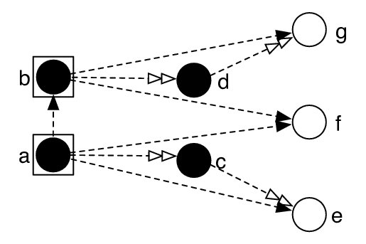
It is trivial that for standard patterns with flow, the quantum computation depth is the same as the flow depth. However for wild patterns, the quantum computation depth cannot be dissociated from the preparation depth (the $E$ commands being interspersed within the pattern). In order to define this combined preparation and quantum depth, we define the execution digraph in a similar way as Definition 3.2, but we add the $E$ commands to the execution digraph. Then the depth of a wild pattern is the longest path in the execution digraph except that we allow a sequence of $E$ commands to be parallelized, the depth of such a sequence being given by the results of Section 3.1.

4 Standardization reduces depth

In this Section, we refer to the combined preparation and quantum depth of a pattern as its depth. Intuitively, we would expect that standardization could only potentially decrease this depth. This is because by standardizing, we benefit from the fact that there is a single entanglement graph to consider. Also, corrections are propagated to the end and applied only on output qubits, hence potentially fewer operations are needed. On the other hand, standardization creates dependent measurements. The following theorem (which is general and independent of the flow construction) confirms all these observations. Let $\mathcal{P}\Rightarrow^{\star}\mathcal{P}^{\prime}$ denote the fact that $\mathcal{P^{\prime}}$ is obtained from $\mathcal{P}$ by applying a finite sequence of rewrite rules given by equations (1)–(4).

Theorem 4.1.

Whenever $\mathcal{P}\Rightarrow^{\star}\mathcal{P^{\prime}}$ where $P^{\prime}$ is in standard form, the depth of $\mathcal{P^{\prime}}$ is less than or equal to the depth of $\mathcal{P}$ .

Proof.

First, we apply the free commutation rules on those commands operating on disjoint sets of qubits (see Appendix B) to $\mathcal{P}$ to obtain $\mathcal{P^{*}}$ as a sequence of standard patterns. The depth as defined by the execution digraph is not affected by this procedure, and $\mathcal{P^{*}}$ depth is actually the sum of the depths of its standard parts. Thus it is sufficient to show that standardization of a wild pattern $\mathcal{P}$ , containing two parts in standard form, say $\mathcal{P}=C^{2}M^{2}E^{2}C^{1}M^{1}E^{1}$ (where some or all of the parts may be empty), does not increase its depth. The theorem then follows by induction.

Step 1. (The $E$ ’s)

We show how the re-writing rules are used to bring the pattern $\mathcal{P}=C^{2}M^{2}E^{2}C^{1}M^{1}E^{1}$ to $\mathcal{P^{\prime}}=C^{2}M^{2}C^{1^{\prime}}M^{1}E^{2}E^{1}$ and that by doing so, the depth of $\mathcal{P^{\prime}}$ is no greater than that of $\mathcal{P}$ . The result holds trivially, if $E^{2}$ is empty. Otherwise, for every command $E_{ij}\in E^{2}$ , commute it to the right-hand side of the pattern by doing the following:

1.

If $C^{1}$ contains $Z_{i}$ or $Z_{j}$ corrections, but no $X_{i}$ or $X_{j}$ corrections, we apply the rewriting rule $E_{ij}Z_{i}^{s}\Rightarrow Z_{i}^{s}E_{ij}$ and hence the depth does not increase. We then complete the commutation by applying the free commutation rules.
2.

If $C^{1}$ contains $X_{i}$ or $X_{j}$ , then the rewriting rule $E_{ij}X_{i}^{s}\Rightarrow X_{i}^{s}Z_{j}^{s}E_{ij}$ applies. Here, the command $X_{i}^{s}$ has an $s$ dependency, which obviously cannot contain $i$ or $j$ , since these qubits haven’t been measured yet. Since $X_{i}^{s}$ and $Z_{i}^{s}$ do not depend on each other, the addition of the extra correction does not contribute to the depth.We then complete the commutation by applying the free commutation rules.

Finally, consider the entanglement graph for $E^{1}E^{2}$ . Since $\chi^{\prime}(E^{1}\cup E^{2})\leq\chi^{\prime}(E^{1})+\chi^{\prime}(E^{2})$ , clearly, the preparation depth for $E^{1}\cup E^{1}$ cannot be any greater than the depth of preparation for $E^{1}$ plus $E^{2}$ . Also, as an extra bonus, since $E_{ij}$ is self-inverse, if $E^{1}$ and $E^{2}$ happen to have common commands, they will cancel out.

Step 2. (The $M$ ’s)

We will show how the free commutation rules and the re-writing rules are used to bring the pattern $\mathcal{P^{\prime}}=C^{2}M^{2}C^{1^{\prime}}M^{1}E^{2}E^{1}$ to its standard form $\mathcal{P^{\prime\prime}}=C^{2}C^{1^{\prime\prime}}M^{2^{\prime}}M^{1}E^{2}E^{1}$ and that doing so, the depth of $\mathcal{P^{\prime\prime}}$ is no greater than that of $\mathcal{P^{\prime}}$ .

1.

Consider a command ${}_{t}[M_{i}^{\alpha}]^{s}\in M^{2}$ . If $C^{1^{\prime}}$ does not contain any commands acting on qubit $i$ , then ${}_{t}[M_{i}^{\alpha}]^{s}$ freely commutes in $C^{1^{\prime}}$ , hence we have commuted ${}_{t}[M_{i}^{\alpha}]^{s}$ to the right-hand side of $C^{1^{\prime}}$ , and clearly the sum of the depths of the patterns $C^{2}M^{2}$ and $C^{1^{\prime}}M^{1}E^{2}E^{1}$ is greater than or equal to the depth of the pattern $C^{2}C^{1^{\prime}}M^{2}M^{1}E^{2}E^{1}$ .
2.

Otherwise, we apply the rewrite rules of equations (3) and (4). In the execution digraph, both of these rules correspond to an edge contraction ²² 2 The contraction of edge $e=(x,y)$ of a graph $G$ is obtained by contracting the edge $e$ into a new vertex, $v_{e}$ , which becomes adjacent to all the former neighbours of $x$ and $y$ . This definition also applies to digraphs.. The depth of the execution digraph obviously does not increase by contracting any of its edges. Hence, after the applicable edge contractions, we can commute the commands as above, yielding a pattern of smaller or equal depth. ∎

Theorem 4.1 shows us that in order to improve the parallel run-time of the pattern, we should implement the standard form of the pattern. We also know that standardization can be performed in polynomial time [17]. Thus in the remainder of the paper, we will only consider standard patterns, which also allows us to consider the preparation depth separately from the quantum computation depth. Combined with Theorem 5.1 of the next section, we note that the most efficient form for the implementation of a pattern is also the signal-shifted form.

5 Signal shifting reduces depth

The signal shifting rules (Equations (5)–(8)) tell us how we can push the $Z$ dependencies of a pattern all the way to the end, which can then decrease the quantum depth of a pattern in standard form. We first present an example and then prove the result, which is also general and independent of the flow construction.

Example. Consider the standard pattern given in Equation (10). After, signal shifting, we obtain the following equivalent pattern:

\begin{array}[c]{lllllllllllllll}&&Z_{g}^{s_{b}}X_{g}^{s_{d}}Z_{f}^{s_{b}}Z_{f}^{s_{a}}Z_{e}^{s_{a}}X_{e}^{s_{c}}[{M}_{d}^{\delta}]^{s_{b}}[{M}_{c}^{\gamma}]^{s_{a}}\framebox{${}_{s_{a}}[{M}_{b}^{\beta}]$}{M}_{a}^{\alpha}E_{G}\\ &\Rightarrow_{\mbox{Eq.}(\ref{e-signal1})}&Z_{g}^{s_{b}}X_{g}^{s_{d}}Z_{f}^{s_{b}}Z_{f}^{s_{a}}Z_{e}^{s_{a}}X_{e}^{s_{c}}[{M}_{d}^{\delta}]^{s_{b}}[{M}_{c}^{\gamma}]^{s_{a}}S_{b}^{s_{a}}{M}_{b}^{\beta}{M}_{a}^{\alpha}E_{G}\\ &\Rightarrow&Z_{g}^{s_{b}}X_{g}^{s_{d}}Z_{f}^{s_{b}}Z_{f}^{s_{a}}Z_{e}^{s_{a}}X_{e}^{s_{c}}\framebox{$[{M}_{d}^{\delta}]^{s_{b}}S_{b}^{s_{a}}$}[{M}_{c}^{\gamma}]^{s_{a}}{M}_{b}^{\beta}{M}_{a}^{\alpha}E_{G}\\ &\Rightarrow_{\mbox{Eq.}(\ref{e-signal4})}&Z_{g}^{s_{b}}X_{g}^{s_{d}}\framebox{$Z_{f}^{s_{b}}S_{b}^{s_{a}}$}Z_{f}^{s_{a}}Z_{e}^{s_{a}}X_{e}^{s_{c}}[{M}_{d}^{\delta}]^{s_{b}+s_{a}}[{M}_{c}^{\gamma}]^{s_{a}}{M}_{b}^{\beta}{M}_{a}^{\alpha}E_{G}\\ &\Rightarrow_{\mbox{Eq.}(\ref{e-signal3})}&\framebox{$Z_{g}^{s_{b}}S_{b}^{s_{a}}$}X_{g}^{s_{d}}Z_{f}^{s_{b}+s_{a}}Z_{f}^{s_{a}}Z_{e}^{s_{a}}X_{e}^{s_{c}}[{M}_{d}^{\delta}]^{s_{b}+s_{a}}[{M}_{c}^{\gamma}]^{s_{a}}{M}_{b}^{\beta}{M}_{a}^{\alpha}E_{G}\\ &\Rightarrow_{\mbox{Eq.}(\ref{e-signal3})}&Z_{g}^{s_{b}+s_{a}}X_{g}^{s_{d}}Z_{f}^{s_{b}}Z_{e}^{s_{a}}X_{e}^{s_{c}}[{M}_{d}^{\delta}]^{s_{b}+s_{a}}[{M}_{c}^{\gamma}]^{s_{a}}{M}_{b}^{\beta}{M}_{a}^{\alpha}E_{G}\\ \end{array}

where boxes represent terms to be rewritten. Now in the new execution digraph (Figure 3) the longest path has only three vertices, hence signal shifting has decreased the depth by one.

The following theorem states that, in general, signal shifting does not increase the depth of a standard pattern. As we have seen above, it can sometimes decrease it.

Theorem 5.1.

Signal shifting for a standard pattern does not increase the depth.

Proof.

Let $\mathcal{P}$ be a pattern in standard form and suppose that $\mathcal{P}$ includes a command ${}_{t}[M_{i}^{\alpha}]^{s}$ which generates the signal shifting command $S_{i}^{t}$ . Let $\mathcal{P^{\prime}}$ be the pattern that corresponds to the pattern after the signal $S_{i}^{t}$ has been shifted. Let $D$ be the execution digraph for $\mathcal{P}$ and let $D^{\prime}$ be the execution digraph for $\mathcal{P^{\prime}}$ . We want to show that the length of a critical path of $D^{\prime}$ is no greater than the length of a critical path of $D$ .

Suppose that the domain of $s$ in ${}_{t}[M_{i}^{\alpha}]^{s}$ is $s_{1},s_{2},\ldots,s_{n}$ and that the domain of $t$ is $t_{1},t_{2},\ldots,t_{m}$ . Consider all the commands that appear after ${}_{t}[M_{i}^{\alpha}]^{s}$ in $\mathcal{P}$ and that have an $i$ dependency; denote these commands $C_{a_{1}}^{i},C_{a_{2}}^{i},\ldots,C_{a_{k}}^{i}$ (these are either corrections or measurements). We will show that the depth does not increase when we shift the signal $S_{i}^{t}$ passed all the $C_{a}^{i}$ ’s.

Consider the arcs in $D$ that represent the dependencies between the measurement ${}{{}_{t}}[M_{i}^{\alpha}]^{s}$ and measurements of qubits $t_{1},t_{2},\ldots,t_{m}$ ; these are the arcs $t_{j}i$ (for $j=1\ldots m$ ) and we will call these the old arcs. So the old arcs represent $Z$ -dependencies for the ${}{{}_{t}}[M_{i}^{\alpha}]^{s}$ measurement. These are precisely those that create signal shifting commands, since ${}{{}_{t}}[M_{i}^{\alpha}]^{s}\Rightarrow S_{i}^{t}\,[M_{i}^{\alpha}]^{s}$ .

Now consider the arcs in $D^{\prime}$ that represent the dependencies between the measurement of qubit $t_{j}$ , $M_{t_{j}}$ $(j=1\ldots m)$ and the measurements and corrections that have an $i$ dependency, $C_{a_{x}}^{i}$ ( $x=1\ldots k$ ). We call these arcs new arcs since they represent the new dependencies created by $S_{i}^{t_{1}},S_{i}^{t_{2}},\ldots,S_{i}^{t_{n}}$ by the signal shifting rules given in equations (5)–(8).

Indeed, when we apply signal shifting to $\mathcal{P}$ , we get rid of all the dependencies represented by old arcs, yet we add all the dependencies represented by new arcs. These are the only differences between the execution digraphs $D$ and $D^{\prime}$ .

If all new arcs are already in $D$ (this could be the case if all the dependencies were present before signal shifting), the graph $D^{\prime}$ cannot have a longer critical path than $D$ and we are done. Otherwise, suppose for a contradiction that the length of a critical path in $D^{\prime}$ is greater than the length of a critical path in $D$ . Since $D^{\prime}$ differs from $D$ only by the removal of all the old arcs and the addition of all the new arcs, the only way for $D^{\prime}$ to have a longer critical path than $D$ would be for this critical path to include a new arc, say $t_{j}a_{k}$ (obviously, the removal of the old arcs in $D^{\prime}$ cannot contribute to a longer critical path.) But if such a critical path exists in $D^{\prime}$ , then $D$ admits a longer critical path, namely the same critical path in $D^{\prime}$ , but with arcs $t_{j}i$ and $ia_{k}$ instead of arc $t_{j}a_{k}$ . This contradiction proves our claim. ∎

There is a tradeoff when we perform signal shifting, as it can increase the classical depth. However, as we will show later, the classical depth is at most $O(\log(n))$ at each layer, where $n$ is the number of measured qubits (Proposition 6.6) and hence the tradeoff is beneficial, especially from the point of view that classical computation is cheap and reliable, compared to quantum computation that is expensive, error-prone and subject to decoherence.

6 Flow and pattern depth

While the results of Sections 4 and 5 deal with the depth of any pattern, we now focus our attention on the depth of patterns with flow. The flow condition is sufficient but not necessary for determinism [29], however the class of patterns with flow is still an interesting class of patterns, as it is universal for quantum computing, closed under composition and more importantly our translation from circuits to patterns in Section 7 always yields a pattern with flow. For the rest of the paper we consider only patterns with flow.

It is known that for patterns with flow and equal input and output number of qubits, i.e. those implementing a unitary operator, the flow, if it exists, is unique [25]. From this, we obtain an upper bound on the quantum computation depth directly from the underlying geometry. We first define an important notion of influencing paths for geometries.

Definition 6.1.

Let $(f,\preceq)$ be the flow of a geometry $(G,I,O)$ . Any input-output path in $G$ that starts with a flow edge and has no two consecutive non-flow edges is called an influencing path.

The following are examples of several influencing paths in the geometry with flow of Figure 1 in Section 3.2:

\begin{array}[c]{lllllllllllllll}ace,acf,acbdf,acbdg\,.\end{array}

Proposition 6.2.

Let $a$ and $b$ be two qubits in a standard pattern with flow. If $b$ depends on $a$ , then $a$ appears before $b$ on a common influencing path, and this hold both before and after signal shifting.

Proof.

This is a consequence of the Flow Theorem. Recall that before signal shifting, a measurement at a qubit $j$ is $X$ -dependent on the result of a measurement at another qubit $i$ if and only if $j=f(i)$ that is, a flow edge between qubits $i$ and $j$ . Also a measurement at a qubit $k$ is $Z$ -dependent on the result of a measurement at another qubit $i$ if and only if $j=f(i)$ and $k$ is connected to $j$ , that is a non-flow edge between qubits $j$ and $k$ connected to a flow edge between qubits $i$ and $j$ . Therefore signal shifting creates new dependencies only through influencing paths. Hence if qubit $b$ depends on qubit $a$ , it is either via a direct $X$ or $Z$ dependency or due to a sequence of dependencies after signal shifting, in all the cases $a$ and $b$ must be on a common influencing path. ∎

Proposition 6.2 tells us that in order to compute the quantum depth of a standard pattern with flow (to which we either have or haven’t applied signal shifting), it suffices to consider the depth along influencing paths. Note that after signal shifting, $Z$ -dependencies coming from the non-flow edges on an influencing path no longer contribute to the pattern depth, as the dependencies that they represent are pushed to the final correction on an output qubit. On the other hand, signal shifting can create new $X$ -dependencies. The following proposition presents an upper bound on the effect of signal shifting on the pattern depth.

Proposition 6.3.

Let $\mathcal{P}$ be a pattern with flow where standardization and signal shifting have been performed. Then the maximum number of flow edges, minus the number of the non-flow edges on such path (maximum taken over all possible influencing paths), plus 1 is an upper bound for the depth of the pattern.

Proof.

We show that for any influencing path, its number of flow edges minus the non-flow edges gives an upper bound on its depth. Then, by Proposition 6.2, it suffices to find the largest number of flow edges along any influencing path in order to have an upper bound on the depth. We add $1$ to this depth since the depth is the number of vertices of such path, and not the number of edges.

Consider an influencing path $I$ . The flow edges represent $X$ -dependencies hence each flow edge in a sequence of consecutive flow edges contributes to the depth along $I$ . Now, consider a configuration with a non-flow edge as shown in Figure 4. Before signal shifting, the dependent measurements on qubits $i$ , $j$ , $k$ and $\ell$ are given as follows (see Equation (9)) where $A,B$ and $C$ stand for general signals not including $s_{i},s_{j},s_{k}$ and $s_{\ell}$

\begin{array}[c]{lllllllllllllll}\dots{}_{D}[{M}_{\ell}^{\alpha_{\ell}}]^{s_{k}}\,{}_{C+s_{i}}[{M}_{k}^{\alpha_{k}}]^{B}\,{}_{A}[{M}_{j}^{\alpha_{j}}]^{s_{i}}\dots\end{array}

and after signal shifting we have

\begin{array}[c]{lllllllllllllll}&&\cdots{}_{D}[{M}_{\ell}^{\alpha_{\ell}}]^{s_{k}}{}_{C+\framebox{$s_{i}$}}[{M}_{k}^{\alpha_{k}}]^{B}{}_{A}[{M}_{j}^{\alpha_{j}}]^{s_{i}}\cdots\\ &\Rightarrow&\cdots\framebox{${}_{D}[{M}_{\ell}^{\alpha_{\ell}}]^{s_{k}}S_{k}^{s_{i}}$}{}_{C}[{M}_{k}^{\alpha_{k}}]^{B}{}_{A}[{M}_{j}^{\alpha_{j}}]^{s_{i}}\cdots\\ &\Rightarrow&\cdots S_{k}^{s_{i}}{}_{D}[{M}_{\ell}^{\alpha_{\ell}}]^{s_{k}+s_{i}}{}_{C}[{M}_{k}^{\alpha_{k}}]^{B}{}_{A}[{M}_{j}^{\alpha_{j}}]^{s_{i}}\cdots\\ \end{array}

Therefore qubits $j$ and $\ell$ are in the same layer. In other words, after signal shifting, the first flow edge after every non-flow edge does not contribute to the depth of the pattern. Also, any new $X$ -dependency created with signal shifting will not increase the depth. Hence from the total number of the flow edges on an influencing path we need to subtract the number of non-flow edges. ∎

So far we have not taken into account the information about the angles, which is why our bounds are not tight. We first describe the effect of the Pauli measurements on depth. The following identities are useful

	$\displaystyle{M}_{i}^{\frac{\pi}{2}}X_{i}^{s}$	$\displaystyle={M}_{i}^{\frac{\pi}{2}}Z_{i}^{s}$		(11)
	$\displaystyle{M}_{i}^{0}X_{i}^{s}$	$\displaystyle={M}_{i}^{0}$		(12)

According to Equation (11), when a qubit $i$ is measured with angle $\frac{\pi}{2}$ (Pauli $Y$ measurement), then any $X$ -dependency on this qubit is the same as a $Z$ -dependency. But after signal shifting, this $Z$ -dependency does not directly contribute to the depth and hence we might obtain a smaller depth. Furthermore, there exists a special case where if qubit $i$ is not an input qubit and also not the flow image of any other vertex ( $\forall j:i\not=f(j)$ ) and qubit $i$ is measured with $\frac{\pi}{2}$ , then one can permit in the Flow Theorem, to have $f(i)=i$ and hence we will have one less flow edge [19]. This allows an influencing path to have a loop edge on this particular vertex measured with Pauli $Y$ and hence the influencing path will not start with an input qubit. In the rest of the paper, we consider only this extended notion of influencing path that takes into account the angles of measurement. When we want to emphasize this extended definition, we will refer to Pauli influencing paths.

According to Equation (12), another special case is when qubit $i$ is measured with angle $0$ (Pauli $X$ measurement), then any $X$ -correction on qubit $i$ can be ignored and in fact qubit $i$ can be put at the first level of measurement. Consequently, again the flow depth can become smaller. By adding equations (11) and (12) to the Flow Theorem, the proof still works [19] and we get a potential improvement on the depth complexity. We refer to this procedure as Pauli simplification. Another way of realizing these special cases is that after signal shifting, the Pauli measurements become independent measurements and hence can all be performed at the first level of the partial order. Hence in computing the depth of a pattern with flow after signal shifting is performed, one should disregard the Pauli measurements:

Proposition 6.4.

Let $\mathcal{P}$ be a pattern with flow where standardization, Pauli simplification and signal shifting have been performed. Let $I_{i}$ be a Pauli influencing path of $\mathcal{P}$ , denote by $e_{i}$ the number of the flow edges, by $n_{i}$ the number of non-flow edges, by $p_{i}$ number of flow edges pointing to a qubit to be measured with a Pauli measurement and by $\ell_{i}$ the number of loop edges ( $\ell_{i}\in\{0,1\}$ ). Then the depth of the pattern, call it $D_{\mathcal{P}}$ satisfies the following formula:

\begin{array}[c]{lllllllllllllll}D_{\mathcal{P}}\leq\max_{I_{i}}e_{i}-(n_{i}+p_{i}+\ell_{i})+1\,.\end{array}

Proof.

Along any Pauli influencing path, any flow edge pointing to a qubit to be measured by a Pauli $X$ will not require a separate layer (Equation (12)) and for the Pauli $Y$ case, such a flow edge is converted to a $Z$ -dependency (Equation (11)), to be signal shifted as in Corollary 6.3. Also if the influencing path starts with a $Y$ measurement followed by a non-Pauli measurement, we have a loop edge and hence the immediate following non-Pauli measurement can also be put in the first layer and hence we subtract the loop edge from the total depth for this influencing path. ∎

6.1 Classical depth

One issue that has often been overlooked in the literature on MBQC is that computation of the correction exponents as well as the measurement angles contributes to a classical depth [8]. Consider, for example, the case where we have a correction of the form $X_{i}^{s_{1}+s_{2}+\cdots+s_{n}}$ . An efficient implementation would start by classically calculating the parity of the exponent, and then applying the correction if the parity is $1$ . This is also the case for a measurement angle such as $[{M}_{i}^{\alpha}]^{s_{1}+s_{2}+\cdots+s_{n}}$ , where one needs to delay the quantum computation to classically compute the measurement angle. Luckily all these classical delays are of at most $O(\log(n))$ depth, since the parity of $n$ bits can be computed by a divide-and-conquer method in depth $O(\log(n))$ (any polynomial-size parity circuit has depth in $\Omega(\log^{*}\!n)$ [30]). Such a classical computation cost between quantum layers is negligible, but it still exists. Actually, depending on the underlying geometry of a pattern, this classical processing sometimes requires only constant depth. This can be easily seen for a pattern with flow.

Lemma 6.5.

Let $\mathcal{P}$ be a standard pattern with flow and geometry $G$ , before signal shifting has been performed. The depth of the classical processing required between quantum layers is in $O(\log\Delta(G))$ .

Proof.

From the Flow Theorem, we know that each measurement at qubit $i$ has at most one $X$ -dependency from one of its neighbours in $G$ and the rest of the neighbours of $i$ contribute at most one $Z$ -dependency. Hence the depth for the classical computation required for calculating the measurement angles at qubit $i$ is in $O(\log(\deg(i)))$ . Therefore, at each qubit, the classical depth is in $O(\log\Delta(G))$ . ∎

Therefore, for a simple geometry such as the cluster state with maximum degree 4, all classical computation is constant. On the other hand, signal shifting which is essential for decreasing the quantum depth, will increase the classical depth. We now present an explicit quantum-classical tradeoff for patterns with flow. But first, we need to define a partial influencing path: let $v$ be a node in geometry $G$ . Then an $I$ - $v$ partial influencing path is a path in $G$ that starts with a flow edge at an input node in $I$ , ends with a flow edge at node $v$ , and contains no consecutive non-flow edges.

Proposition 6.6.

Let $\mathcal{P}$ be a pattern with flow where standardization and signal shifting have been performed. Fix a node $v$ in the underlying geometry $G$ and let $I_{v}$ be the set of all partial influencing paths, from an input qubit $i$ to the node $v$ . (If $v$ is an output qubit we consider all the influencing paths instead.) Let $N_{v}$ be the set of vertices that are on any path in $I_{v}$ . Then the classical depth of the required classical computation for computing the angles of measurement command or the exponent of correction command at $v$ is in $O(\log\lvert N_{v}\rvert)$ .

Proof.

In the proof of Lemma 6.5, we saw how the Flow Theorem tells us which dependencies are applied to a qubit $v$ . Once signal shifting has been done, the dependencies are modified, but they still propagate only through influencing paths. In fact for the case of $v$ being a measured qubit, after signal shifting only the $X$ -dependencies remain and therefore we need to consider only the partial influencing paths. Hence there are at most $\lvert N_{v}\rvert$ dependencies at $v$ ; the parity of these dependencies can be computed in classical depth $O(\log\lvert N_{v}\rvert)$ . ∎

Note that $N_{v}$ is upper bounded by the total number of qubits in the pattern. However for a particular geometry and angles of measurement, it can be smaller. For example, consider a pattern with $n$ input qubits and a geometry of a full cluster state of size $n$ times width equal to $D$ , as shown in Figure 5. Then from the above proposition, we conclude that the classical depth is in $O(\log(D)$ : for any given qubit $i$ only the $O(D^{2})$ qubits siting on the pyramid with qubit $i$ as the top of the pyramid, will contribute to the depth complexity of the command to be performed at qubit $i$ (see Figure 5). Therefore, for $D\in O(\log(n))$ , we obtain small classical depth of size $O(\log(\log(n)))$ , whereas the total number of the qubits in the pattern is in $O(n\log(n))$ .

7 Circuits and measurement patterns

Having built all the required tools, we can now turn our attention to the main focus of the paper on parallelizing quantum circuits. To this end we give a method to translate a quantum circuit to a pattern (Section 7.1) and vice-versa (Section 7.2), where standardization, signal shifting and Pauli simplifications on the obtained pattern leads to a more parallel circuit. We also present the exact tradeoff for the transformations. Furthermore, our construction allows us to see influencing paths directly in the quantum circuit so that the pattern depth characterization results given in Section 8 can be directly applied to circuits.

We fix the universal family of gates to be $\mathfrak{U}=\{\mathop{\wedge}\hskip-1.72218ptZ,J(\alpha)\}$ :

\begin{array}[c]{lllllllllllllll}\mathop{\wedge}\hskip-1.72218ptZ=\left(\begin{matrix}1&0&0&0\\ 0&1&0&0\\ 0&0&1&0\\ 0&0&0&-1\end{matrix}\right),\,\,J(\alpha)=\frac{1}{\sqrt{2}}\left(\begin{matrix}1&e^{i\alpha}\\ 1&-e^{i\alpha}\end{matrix}\right)\,.\end{array}

In [31, 32] it was shown that this family is universal for the circuit model since every single qubit unitary operator can be written in terms of $J(\alpha)$ :

\begin{array}[c]{lllllllllllllll}U=e^{i\alpha}J(0)J(\beta)J(\gamma)J(\delta)\end{array}

In addition, they lead to simple generating patterns:

	$\displaystyle J(\alpha)$	$\displaystyle:=X_{2}^{s_{1}}{M}_{1}^{{-\alpha}}E_{12}$		(13)
	$\displaystyle\mathop{\wedge}\hskip-1.72218pt{Z}$	$\displaystyle:=E_{12}\,.$		(14)

Hence this family of unitaries is a good choice for translation between circuits and patterns and any other universal family can be replaced by this one with constant overhead. In the rest of the paper, whenever the angle $\alpha$ is not important, we simply refer to a $J(\alpha)$ gate as a $J$ gate.

7.1 From circuits to patterns

The original universality proof for MBQC already contained a method to translate a quantum circuit containing arbitrary 1-qubit rotations and control-not gates to a pattern [14]. Here, we give an alternate method for the translation of a given circuit to a standard pattern in the MBQC to attempt to reduce the quantum depth. We give the exact tradeoff in terms of the number of auxiliary qubits and depth.

Recall that $\mathop{\wedge}\hskip-1.72218ptZ$ is self-inverse and symmetric, hence any circuit that contains consecutive $\mathop{\wedge}\hskip-1.72218ptZ$ gates acting on the same qubits can be simplified. In what follows, we suppose that this simplification has been performed.

Definition 7.1.

Let $C$ be a circuit of $\mathop{\wedge}\hskip-1.72218ptZ$ and $J$ gates on $n$ logical qubits. The corresponding standard pattern $\mathcal{P}$ is obtained by replacing each gate in $C$ with its corresponding pattern given by equations (13) and (14), and then performing standardization and signal shifting.

To present the exact tradeoff for the above translation, in particular to prove that the quantum depth cannot increase, we construct directly the underlying geometry of a given circuit. Following the literature, we refer to the circuit qubits as logical qubits. Other qubits that are added during construction of the entanglement graph will be referred to as auxiliary qubits.

Definition 7.2.

Let $C$ be a circuit of $\mathop{\wedge}\hskip-1.72218ptZ$ and $J$ gates on $n$ logical qubits. The labelled entanglement graph $G_{C}$ is constructed as a layer that is initially built on top of the circuit $C$ by the following steps (see also the example of Figure 6).

1.

Replace each $\mathop{\wedge}\hskip-1.72218ptZ$ gate on logical qubits $i$ and $j$ with a vertical edge between two vertices: one on the $i^{\text{th}}$ wire and one on the $j^{\text{th}}$ wire. Label both vertices Input/Output. Replace each $J$ gate on a logical qubit $i$ with an horizontal edge between two vertices on the $i^{\text{th}}$ wire, label the left vertex Input and the right vertex Output.
2.

To connect the above components, on each wire, start from the left and contract consecutive non-adjacent vertices as follows (the contraction of vertices $v_{1}$ and $v_{2}$ of a graph $G$ is obtained by replacing $v_{1}$ and $v_{2}$ by a single vertex $v$ , which is adjacent to all the former neighbours of $v_{1}$ and $v_{2}$ ):
- –
  
  Two vertices labelled Input/Output are contracted as one vertex with Input/Output label;
- –
  
  A vertex labelled Input/Output and a vertex labelled Input are contracted as one vertex with Input label;
- –
  
  A vertex labelled Output and a vertex labelled Input/Output are contracted as one vertex with Output label;
- –
  
  Two vertices labelled Output and Input are contracted as one vertex with auxiliary label.

It is easy to verify the following proposition that justifies the above construction.

Proposition 7.3.

The graph $G_{C}$ obtained from Definition 7.2 is the entanglement graph for the measurement pattern that is obtained from Definition 7.1. Furthermore, input-output paths of vertices sitting on the same wire define the flow of $G_{C}$ .

Proof.

Standardization does not change the underlying entanglement graph, hence it follows that $G_{C}$ is indeed the entanglement graph for the measurement pattern. By Theorem 10 of [25], for the case that $\lvert I\rvert=\lvert O\rvert$ , a collection of vertex-disjoint $I-O$ paths in $G_{C}$ define its flows. Therefore, input-output paths of vertices sitting on the same wire define the flow of $G_{C}$ . ∎

In order to obtain a full pattern corresponding to the circuit $C$ , one needs to add measurement commands with angles being the same angles of the $J(\alpha)$ gates. These angles are assigned to the qubits labelled Input in Step (1) of the construction of Definition 7.2. The dependency structure is the one obtained from the Flow Theorem.

Proposition 7.4.

Let $C$ be a quantum circuit on $n$ logical qubits with only $\mathop{\wedge}\hskip-1.72218ptZ$ and $J$ gates. Let $G_{2}$ be the number of $J$ gates and $D(n)$ the circuit depth. The corresponding pattern $\mathcal{P}$ given by Definition 7.1 has $n+G_{2}$ qubits, $G_{2}$ measurement commands, $n$ corrections commands, and depth smaller than or equal to $D(n)$ .

Proof.

The proof is based on construction of Definition 7.2, which is obtained from replacing the patterns from equations (13) and (14) for $J$ and $\mathop{\wedge}\hskip-1.72218ptZ$ gates and then performing the standardization procedure. It is clear from the construction that we start with $n$ qubits corresponding to each wire, then any $\mathop{\wedge}\hskip-1.72218ptZ$ connects the existing qubits (wires) and hence will not add to the total number of qubits. On the other hand any $J$ gate extends the wire by adding a new qubit. This leads to the total number of $n+G_{2}$ qubits for the pattern. There are $G_{2}$ measurement commands since all but $n$ qubits are measured. Since $C$ has depth $D(n)$ , any influencing path in $\mathcal{P}$ has at most $D(n)$ flow edges. Hence the theorem is obtained from Proposition 6.3 after performing signal shifting on the corresponding pattern. ∎

Alternatively, for a given circuit, one can use another construction to obtain a corresponding pattern with cluster geometry, hence to achieve constant depth for the graph preparation stage. Naturally, the price is to have more qubits. First note that the following pattern implements teleportation from input qubit $i$ to output qubit $k$ that is simply the identity map (see Figure 7):

\displaystyle X_{k}^{s_{j}}Z_{k}^{s_{i}}{M}_{j}^{0}{M}_{i}^{0}E_{jk}E_{ij}

(15)

Now, if before Step (2) of the construction of Definition 7.2, we insert the teleportation pattern between any two consecutive $\mathop{\wedge}\hskip-1.72218ptZ$ acting on a common wire, then the degree of each vertex remains less than 4 as desired. We will refer to this graph as the cluster graph, ${GC}_{C}$ . In order to compute the number of qubits for the pattern obtained from this new construction, consider the positions in the circuit where two $\mathop{\wedge}\hskip-1.72218ptZ$ appear after each other. These are the places where we need to apply the above teleportation pattern to keep the degree less than 4. With this construction, the depth of the pattern does not increase by more than a multiplicative constant. Therefore we have:

Lemma 7.5.

Let $C$ be a quantum circuit on $n$ qubits with only $\mathop{\wedge}\hskip-1.72218ptZ$ and $J$ gates. Let $G_{2}$ be the number of $J$ gates, $s$ the size of $C$ and $m$ the number of positions in $C$ where two $\mathop{\wedge}\hskip-1.72218ptZ$ appear after each other. Then the pattern $\mathcal{P}$ with the cluster graph construction (obtained as in Proposition 7.3 with the addition of the teleportation pattern above) has $n+G_{2}+m\in O(n+s)$ qubits and depth in $O(D(n))$ .

In what follows, we always assume the cluster geometry for patterns corresponding to a circuit and hence the preparation depth is $4$ (Section 3.1).

7.2 From patterns to circuits

The construction of Definition 7.2 can be also used in reverse order to transfer a pattern with flow to a corresponding circuit, where all the auxiliary qubits will be removed and hence by doing so the quantum depth might increase. However, we now show how to obtain another transformation from patterns to circuits where one keeps all the auxiliary qubits. This new construction is simply based on the well-known method of coherently implementing a measurement. Recall that a controlled-unitary operator where the control qubit is measured in the computational basis { ${|}0\rangle,{|}1\rangle$ } can be written as a classical controlled unitary by pushing the measurement before the controlled-unitary operator [9], see Figure 8.

Given a pattern in the standard form, we use the above scheme in the reverse order to convert the classically dependent measurements and corrections, and then push all the independent measurements to the end of the pattern. However since the scheme works only for the computational basis measurement, we have to first simplify all the arbitrary measurements $M^{\alpha}$ . Let $Z(\alpha)$ be the phase gate and $H$ the Hadamard gate (see Appendix B), and let $M^{Z}$ be the computational basis measurement (i.e. Pauli $Z$ measurement). Then we have

\displaystyle M^{\alpha}=M^{\{{|}+_{\alpha}\rangle,{|}-_{\alpha}\rangle\}}=M^{HZ(-\alpha)^{{\dagger}}\{{|}0\rangle,{|}1\rangle\}}=M^{Z}HZ(-\alpha)\,.

(16)

Additionally, we replace any classical $X$ - and $Z$ -dependencies of measurements and any dependent corrections with a sequence of $\mathop{\wedge}\hskip-1.72218ptX$ and $\mathop{\wedge}\hskip-1.72218ptZ$ , which might creates a quantum depth linear in the number of the dependencies, as shown in Figure 9. However to reduce this linear depth, we can use the following result on parallelizing a circuit with only controlled-Pauli gates to logarithmic depth:

Proposition 7.6.

([11]) Circuits on $n$ qubits consisting of controlled-Pauli gates and the Hadamard gate can be parallelized to a circuit with $O(\log n)$ depth and $O(n^{2})$ auxiliary qubits.

We can now formalize the above translation of patterns to circuits.

Definition 7.7.

Let $\mathcal{P}$ be a standard pattern with computational space $(V,I,O)$ , underlying geometry $(G,I,O)$ (where $G$ has a constant maximum degree) and command sequence (after signal shifting):

\begin{array}[c]{lllllllllllllll}\cdots C_{j}^{C_{j}}\cdots[{M}_{i}^{\alpha_{i}}]^{A_{i}}\cdots E_{G}\end{array}

where $A_{i}$ is the set of qubits that the measurement of qubit $i$ depends on, and $C_{j}$ is the set of qubits that the correction of qubit $j$ depends on. Note that due to the signal shifting, we only have $X$ dependencies. The corresponding coherent circuit $C$ with $|I|$ logical qubits and $|V\smallsetminus I|$ auxiliary qubits, is constructed in the following steps (see also Figure 9):

1.

Apply individual Hadamard gates on all the auxiliary qubits.
2.

Apply a sequence of $\mathop{\wedge}\hskip-1.72218ptZ$ gates according to the edges of $G$ .
3.

Replace any dependent measurement $[{M}_{i}^{\alpha_{i}}]^{A_{i}}$ with $M_{i}^{Z}H_{i}Z_{i}(-\alpha)\mathop{\wedge}\hskip-1.72218pt_{A_{i},i}X$ where $\mathop{\wedge}\hskip-1.72218pt_{A,i}X$ is a sequence of controlled-not with control qubits in $A$ and target qubit $i$ . Note that since the $M^{Z}$ is independent and can be pushed to the end of the corresponding wire it can be discarded.
4.

Replace any dependent correction $X_{j}^{C_{j}}$ with $\mathop{\wedge}\hskip-1.72218pt_{C_{i},i}X$ and $Z_{j}^{C_{j}}$ with $\mathop{\wedge}\hskip-1.72218pt_{C_{i},i}Z$ .
5.

Replace the joint sequence of added $\mathop{\wedge}\hskip-1.72218ptX$ and $\mathop{\wedge}\hskip-1.72218ptZ$ in steps 3 and 4 with the parallel form obtained from Proposition 7.6.

Lemma 7.8.

Let $\mathcal{P}$ be a standard pattern with computational space $(V,I,O)$ and underlying geometry $(G,I,O)$ (where $G$ has a constant maximum degree). Let $t=\lvert V\smallsetminus O\rvert$ be the number of measured qubits and let $d$ be the quantum computation depth of $\mathcal{P}$ . Then the corresponding coherent circuit $C$ obtained from Definition 7.7 has $\lvert I\rvert$ logical qubits, $O(t^{3})$ auxiliary qubits and depth in $O(d\log t)$ .

Proof.

We examine the cost at each step of the construction of Definition 7.7. Steps 1 and 2 add a constant to the depth of $C$ . At step 3, each measurement has as most $t$ dependencies, which, in step 5 translates to $O(\log t)$ depth with $O(t^{2})$ auxiliary qubits. At step 4, each output qubit has at most $t$ dependencies, which again in step 5 translates to $O(\log t)$ depth with $O(t^{2})$ auxiliary qubits. Since the depth of $\mathcal{P}$ is $d$ , the total depth of $C$ is in $O(d\log t)$ , with $O(t^{3})$ auxiliary qubits. ∎

Note that the logarithmic increase in the depth of $C$ is due to the fact that the circuit model does not exploit any classical dependencies. Thus the classical computation of the measurement angles and corrections in $\mathcal{P}$ contributes to the quantum depth in $C$ .

One can combine the forward and backward construction from circuit to patterns to obtain an automated rewriting system for the circuit which can decrease the depth by adding auxiliary qubits. The following theorem gives the tradeoff.

Theorem 7.9.

Let $C$ be a quantum circuit on $n$ qubits with only $\mathop{\wedge}\hskip-1.72218ptZ$ and $J$ gates. Suppose $C$ has size $s$ and depth $D$ . Assume further that $\mathcal{P}$ is the corresponding pattern obtained from the forward translation as in Lemma 7.5 and that $\mathcal{P}$ has quantum depth $D^{\prime}$ (we know that $D^{\prime}\leq D$ ). Then circuit $C^{\prime}$ constructed from $\mathcal{P}$ by Definition 7.7 has $O(s^{3}+n)$ qubits, and depth in $O(D^{\prime}\log s)$ .

Proof.

The first step is to translate $C$ to a pattern $\mathcal{P}$ using Lemma 7.5. The resulting pattern $\mathcal{P}$ has $O(s+n)$ qubits, and quantum depth in $O(D)$ . Then we translate the pattern back to a circuit $C^{\prime}$ using Definition 7.7. By Lemma 7.8, the new circuit has $O(s^{3})$ auxiliary qubits and depth in $O(D^{\prime}\log s)$ . ∎

At first glance it seems like applying Theorem 7.9 to a quantum circuit would not necessary be beneficial, since the number of auxiliary qubits and the depth seem to increase. But note that we have given only upper bounds. As we showed in Section 6, taking into account Pauli simplification and signal shifting can give a significant improvement. In the next section, we give a complete depth characterization for patterns with flow, and then show in Section 8.1 a characterization of those circuits to which applying Theorem 7.9 will necessarily decrease the depth.

8 Depth Characterization

We saw in Section 6 that the main ingredients to obtain a reduced pattern depth are influencing paths, Pauli measurements and signal shifting. In fact, Pauli measurements not only can be performed in the first layer but also they can “reset” the pattern depth along an influencing path. This intuition is formalized in the following lemmas that are essential for our characterization result. In what follows, we deal with sequences of measurements angles, where $N_{i},N_{j},\dots$ represent non-Pauli measurements, $X$ a Pauli $X$ measurement, $Y$ a Pauli $Y$ measurement and $P$ is either $X$ or $Y$ . Furthermore $(\omega)^{*}$ and $(\omega)^{\text{odd}}$ represents respectively, a non-negative and odd number of repetitions of $\omega$ .

Lemma 8.1.

Let $N_{i}$ and $N_{j}$ denote two non-Pauli measurements on a common influencing path $I$ of a standard pattern with flow. Suppose that $N_{i}$ and $N_{j}$ are separated along $I$ with only flow edges, and that the sequence of measurements between $N_{i}$ and $N_{j}$ along $I$ is a sequence of Pauli measurements of the form:

\begin{array}[c]{lllllllllllllll}(X)^{\text{odd}}(Y(X)^{\text{odd}})^{*}\,.\end{array}

Then after signal shifting, there will be no $X$ -dependency between $N_{i}$ and $N_{j}$ .

Proof.

Assume such an $X$ -dependency between $N_{i}$ and $N_{j}$ exists, then it is necessarily due to the fact that during signal shifting, the last Pauli $X$ measurement in the sequence acquires a $Z$ -dependency from $N_{i}$ ; this $Z$ -dependency would then be signal shifted to an $X$ -dependency between $N_{i}$ and $N_{j}$ , since $N_{j}$ has an $X$ -dependency on the last Pauli $X$ measurement. We use a parity argument to show that this never occurs.

First, note that the sequence of Pauli measurements, $(X)^{\text{odd}}(Y(X)^{\text{odd}})^{*}$ is odd. Second, note that through signal shifting, the $Z$ -dependency that originates from $N_{i}$ is shifted only through every even position in the Pauli measurement sequence. Due to the placement of the $Y$ measurements which never occur in an odd position, the special case of the Pauli $Y$ rule (Equation (11)) cannot be applied to change the parity. Hence, the final $X$ measurement in the sequence (which is at an odd position) never sees a $Z$ -dependency from $N_{i}$ (Figure 10). ∎

Lemma 8.2.

Let $N_{i}$ and $N_{j}$ denote two non-Pauli measurements on a common influencing path $I$ of a standard pattern with flow. Suppose that $N_{i}$ and $N_{j}$ are separated along $I$ with only Pauli measurements, i.e. we have the following sequence along $I$ :

\begin{array}[c]{lllllllllllllll}N_{i}\;\mathsf{P}_{1}\;\alpha_{1}\beta_{1}\;\mathsf{P}_{2}\;\alpha_{2}\beta_{2}\;\cdots\;\mathsf{P}_{k}\;N_{j}\,,\end{array}

where $\mathsf{P}_{i}$ is a (possible empty) finite sequence of Pauli measurements and $\alpha_{i}\beta_{i}$ represents the endpoints of a non-flow edge. After signal shifting, there will be no $X$ -dependency due to $I$ between $N_{i}$ and $N_{j}$ if and only if at least one of the $\mathsf{P}_{i}$ sequence is equal to $(X)^{\text{odd}}(Y(X)^{\text{odd}})^{*}$ . This will be also true even if one of the $N_{i}$ or $N_{j}$ are an endpoint of a non-flow edge.

Proof.

First, assume $N_{i}$ and $N_{j}$ are connected with only flow edges (we have the sequence $N_{i}\mathsf{P}N_{j}$ ) and consider the following possible cases for the sequence $\mathsf{P}$ :

(I).

It consists of an even number of Pauli angles. Then there is an $X$ -dependency between $N_{i}$ and $N_{j}$ .
(II).

It consists of an odd number of Pauli angles with at least one $Y$ at an odd position from left to right. Then there is an $X$ -dependency between $N_{i}$ and $N_{j}$ .
(III).

It consists of an odd number of Pauli angles with no $Y$ at any odd position: $(X)^{\text{odd}}(Y(X)^{\text{odd}})^{*}$ . Then there is no $X$ -dependency between $N_{i}$ and $N_{j}$ .

Figure 11 shows how in Case (I), one obtains an $X$ -dependency after signal shifting between $N_{i}$ and $N_{j}$ . Case (II) is also similar, by Pauli simplification, the $X$ -dependency at a $Y$ measurement of an odd position is considered as an $Z$ -dependency and hence we obtain the same scenario as Case (I). Finally, Case (III) is proved in Lemma 8.1.

Now consider the case where there exists a non-flow edge between the non-Pauli angles and neither $N_{i}$ nor $N_{j}$ are an endpoint of a non-flow edge:

\begin{array}[c]{lllllllllllllll}N_{i}\;\mathsf{P}_{1}\;\alpha\beta\;\mathsf{P}_{2}N_{j}\,.\end{array}

According to the Flow Theorem, there is a $Z$ -dependency from the qubit that precedes the qubit assigned to $\alpha$ angle to the qubit with angle $\beta$ . In order to have a sequence of $Z$ dependencies between $N_{i}$ and $\beta$ , $\mathsf{P}_{1}$ must satisfy the conditions of cases (I) or (II) and then similar to the above argument, in order to obtain an $X$ -dependency between $N_{i}$ and $N_{j}$ , $\mathsf{P}_{2}$ must also satisfy the conditions of cases (I) or (II) and hence we obtain the statement of the Lemma. The same argument is valid if either of $N_{i}$ or $N_{j}$ is an endpoint of a non-flow edge. ∎

We can now present our main result on characterization of patterns with a given depth.

Theorem 8.3.

Let $\mathcal{P}$ be a standard pattern with flow and let $I$ be an influencing path of $\mathcal{P}$ . We apply the following simplification rule to the commands along $I$ :

N\,\mathsf{P}_{1}\,\alpha_{1}\beta_{1}\,\mathsf{P}_{2}\,\alpha_{2}\beta_{2}\,\cdots\,\mathsf{P}_{k}\,N\Rightarrow\begin{cases}N\hskip 28.45274pt\text{if}\,\,\,\exists\mathsf{P}_{i}=(X)^{\text{odd}}(Y(X)^{\text{odd}})^{*}\\ NN\qquad\text{otherwise}\,.\end{cases}

where $\mathsf{P}_{i}$ represents a (possible empty) finite sequence of Pauli measurements and $\alpha_{i}\beta_{i}$ represents the endpoints of a non-flow edge. Define the depth of $I$ to be $d+2$ if after the simplification we obtain $\mathsf{P}\,N^{d}\,\mathsf{P}$ and to be $d+1$ if we obtain either $Y\,N^{d}\,\mathsf{P}$ or $N^{d}\,\mathsf{P}$ . Then the quantum depth of $\mathcal{P}$ after Pauli simplification and signal shifting is given by the maximum depth over all influencing paths of $\mathcal{P}$ .

Proof.

Lemma 8.2 justifies the given simplification rule. It is trivial that after applying the rule one will obtain a unique final sequence of the form $\mathsf{P}\,N^{i}\,\mathsf{P}$ on any influencing path and hence the longest sequence of dependent of non-Pauli measurements will have length $i$ and since there is a first layer of Pauli and one final layer of corrections the depth along this path will be $i+2$ . However if the final form is $Y\,N^{i}\,\mathsf{P}$ then there will be no dependency between the Pauli $Y$ and the first non-Pauli $N$ (Equation (11)) and depth is $i+1$ which is also the case for the final form $N^{i}\,\mathsf{P}$ .

According to Proposition 6.2 the pattern depth is the maximum number of the dependent non-Pauli measurements along all the influencing paths and hence it is enough to compute the maximum value of $i$ over all influencing paths. ∎

The above theorem gives a constructive method to obtain a depth $d$ pattern. The main tool being the sequence $(X)^{\text{odd}}(Y(X)^{\text{odd}})^{*}$ , which if it is inserted between two non-Pauli measurements make them independent of each other. On the other hand, any other sequence inserted between non-Pauli angles contributes to the depth and makes the two non-Pauli measurements $X$ -dependent on each other and hence in two different layers of measurement.

We now show as a special case the characterization of patterns with depth 2.

Proposition 8.4.

Let $\mathcal{P}$ be a pattern with flow $f$ , where standardization, Pauli simplification and signal shifting have been performed. The quantum computation depth is equal to 2 if and only if any qubit measured with a non-Pauli angle is not the flow image of any other vertex and hence it is either an input qubit or is connected to a vertex with a loop flow edge.

Proof.

Due to Theorem 8.3, $\mathcal{P}$ has depth 2 if and only if on all the influencing paths, after the simplification rule, we obtain one of the following final forms for the sequence of the measurement angles:

\begin{array}[c]{lllllllllllllll}N\,\mathsf{P}\;\;\;\text{or}\;\;\;Y\,N\,\mathsf{P}\;\;\;\text{or}\;\;\;\mathsf{P}\,.\end{array}

Now consider only those influencing paths with only flow edges, by reverse application of the simplification rules we conclude only input qubits can be measured with a non-Pauli angle or a non-input qubit measured by a non-Pauli measurement should not be the flow image of any other qubit and be connected to a qubit measured with Pauli $Y$ . ∎

Note that this proposition extends the previously know result that patterns with only Pauli measurements have depth 2 [8, 33].

8.1 Parallelizing Circuits

In order to present the pattern depth characterization result directly in terms of the circuit language, we first define the notion of circuit influencing paths.

Definition 8.5.

Let $C$ be a circuit of $\mathop{\wedge}\hskip-1.72218ptZ$ and $J$ gates. A left-to-right path starting at the beginning of a circuit wire and ending at any wire, such that the jumps between wires are done through $\mathop{\wedge}\hskip-1.72218ptZ$ gates is called a circuit influencing path if there exist no two consecutive jumps (see Figure 12).

Recall that for patterns with equal number of input and output qubits, the flow, if it exists, is unique. Hence it is easy to verify that circuit influencing paths defined above are exactly influencing paths of the corresponding pattern via the direct translation given in Section 7. Similar to the pattern case, the circuit depth is characterized in terms of the sequence of $J$ gates appearing on the influencing paths defined below.

Definition 8.6.

Let $I$ be a circuit influencing path of circuit $C$ . The set of $J$ gates over $I$ is defined to be all the consecutive $J$ gates over the wires of the path including the $J$ gates just after a $\mathop{\wedge}\hskip-1.72218ptZ$ gate of a jump, as shown in Figure 12.

Note that, again the above definition is a direct consequence of our transformation between circuits and patterns. Further, define $H^{i}$ to be the single unitary gate

\begin{array}[c]{lllllllllllllll}\frac{1}{\sqrt{2}}\begin{pmatrix}1&-i\\ 1&i\end{pmatrix}\end{array}

implemented by the pattern $X_{2}^{s_{1}}{M}_{1}^{{\frac{\pi}{2}}}E_{12}$ . We also have, $J(0)=H$ and $J(\frac{\pi}{2})=H^{i}$ . We can now present our depth result directly for circuits.

Theorem 8.7.

Let $C$ be a circuit of $\mathop{\wedge}\hskip-1.72218ptZ$ and $J$ gates on $n$ qubits with size $s$ and depth $D$ . Assume that after the following simplification rule on $J$ gates over all circuit influencing paths, we obtain at most $D^{\prime}$ many consecutive $J$ gates:

J\,\mathsf{P}_{1}\,\alpha_{1}\beta_{1}\,\mathsf{P}_{2}\,\alpha_{2}\beta_{2}\,\cdots\,\mathsf{P}_{k}\,J\Rightarrow\begin{cases}J\hskip 28.45274pt\text{if}\,\,\,\exists\mathsf{P}_{i}=(X)^{\text{odd}}(Y(X)^{\text{odd}})^{*}\\ JJ\qquad\text{otherwise}\,.\end{cases}

where $\mathsf{P}_{i}$ represents a (possible empty) finite sequence of $H$ and $H^{i}$ gates and $\alpha_{i}\beta_{i}$ represents the $J$ gates immediately after a $\mathop{\wedge}\hskip-1.72218ptZ$ gate on the underlying circuit influencing path. Then, using the construction of Section 7, circuit $C$ can be parallelized to an equivalent circuit $C^{\prime}$ with depth in $O(D^{\prime}\log(s))$ and size in $O(s^{3}+n)$ .

Proof.

The proof simply follows from theorems 7.9 and 8.3. ∎

Similar to the pattern case, the above theorem gives a constructive method to obtain a depth $d$ circuit. The main tool is the gate sequence

\displaystyle R=(H)^{\text{odd}}(H^{i}(H)^{\text{odd}})^{*}\,,

(17)

which if it is inserted between two $J$ gates over a circuit influencing path will make them to appear in the same layer of the final parallelized circuit.

As an application, consider the quantum circuit in Figure 13 with size in $O(n^{2})$ and depth in $O(n)$ . Theorem 8.7 tell us how to parallelize it to depth in $O(\log(n))$ , while adding $O(n^{6})$ auxiliary qubits. First note that on any circuit influencing path, any two $J$ gates are separated by an $R$ gate (Equation (17)) and hence after the simplification rule, we will have no two consecutive $J$ gates. In other words, the parameter $D^{\prime}$ in Theorem 8.7 is equal to 1 which implies the depth of the parallelized circuit will be in $O(\log(n))$ .

Figure 13: A polynomial-depth circuit where each

J_{ij}

gate has an angle

\in[0,2\pi)

and the

R

gate stands for a sequence of Clifford gates of the form

(H)^{\text{odd}}(H^{i}(H)^{\text{odd}})^{*}

. Theorem 8.7 implies that this circuit can be parallelized to a logarithmic depth circuit.

It is easy to extend the circuit of Figure 13 and still apply Theorem 8.7 to parallelize it to a circuit with depth in $O({\mathbf{poly}}(\log(n)))$ . On each wire, replace $O(\log(n))$ many $J_{ij}$ gates with the following sequence of gates:

\begin{array}[c]{lllllllllllllll}J_{1}\mathsf{P}_{1}J_{2}\mathsf{P}_{2}\dots J_{k}\hskip 14.22636pt\text{with}\hskip 14.22636ptk\in O(\log(n))\end{array}

where $\mathsf{P}_{i}$ is a sequence of $H$ and $H^{i}$ gates of polynomial length. Now the parameter $D^{\prime}$ of Theorem 8.7 is in $O(\log(n))$ and the parallel circuit will have depth in $O(\log^{2}(n))$ .

These set of examples, although somewhat artificially constructed, demonstrate how one might use Theorem 8.7 to construct parallel circuit for a given problem in hand. We finish this section with several other results on circuit parallelization.

Proposition 8.8.

A circuit on $n$ qubits can be parallelized to a pattern of depth 2 via the construction given in Section 7 if and only if it is of the form: a possible sequence of individual phase gates, $Z_{1}(\alpha_{1})\otimes\cdots\otimes Z_{n}(\alpha_{n})$ , followed by an arbitrary poly-size Clifford circuit.

Proof.

It is known that any Clifford gate can be implemented by a pattern with only Pauli $X$ and $Y$ measurements [17, 18]. Hence in one direction, the proof is simply obtained by replacing the phase gates with qubits measured with a non-Pauli angles, that are input qubits. Then by Proposition 8.4, the corresponding pattern has depth 2.

To prove the other direction, let $C$ be a circuit that can be parallelized to a pattern $\mathcal{P}$ with depth 2. Hence from Proposition 8.4 by adding appropriate $(Z(\alpha))^{{\dagger}}$ gates to the beginning of $C$ , we obtain another circuit $C^{\prime}$ that translates to a pattern $\mathcal{P}^{\prime}$ with only Pauli measurements. Now Theorem 4 in [17] implies that $C^{\prime}$ is in the Clifford group and hence $C$ has the desired form. ∎

A simple case of the above proposition is a Clifford circuit, that was known already by [8, 17, 18, 33]. On the other hand, the best known result in terms of depth complexity for the circuit implementing a subgroup of the Clifford group is Proposition 7.6 due to [11]. Using our forward and backward construction of Section 7, we improve this and obtain a general result on circuit depth complexity for the whole Clifford group.

Proposition 8.9.

Any quantum circuit on $n$ qubits of size $s\in{\mathbf{poly}}(n)$ consisting of Clifford gates can be parallelized to a circuit with $O(\log n)$ depth and $O(s^{3}+n)$ auxiliary qubits.

Hence from Propositions 8.8 and 8.9, we see a logarithmic improvement in depth for implementations in the MBQC compared to the circuit model. What we achieve actually is a translation of quantum logarithmic depth in a circuit to constant quantum depth plus classical logarithmic depth in a pattern. We now show that this separation is tight by giving an example of a unitary that can be implemented as a pattern with constant quantum depth, but that must have logarithmic depth in the quantum circuit model.

Lemma 8.10.

Let $U_{p}$ be the parity unitary transformation defined by

\begin{array}[c]{lllllllllllllll}U_{p}\,{|}x_{1},x_{2},\ldots,x_{n}\rangle={|}x_{1},x_{2},\ldots,x_{n-1},\bigoplus_{i=1}^{n}x_{i}\rangle\,.\end{array}

Assume $C$ to be any circuit consisting of 1- and 2-qubit gates that implements this unitary. Then the depth of $C$ is in $\Omega(\log n)$ .

Proof.

Since the state of the last output qubit depends on every input qubit, and the circuit has only 1– and 2–qubit gates, the depth of the circuit must be in $\Omega(\log n)$ . ∎

Figure 14: A logarithmic-depth circuit for parity unitary transformation, where

p=\bigoplus_{i=1}x_{i}

Figure 14 gives a logarithmic depth circuit for $U_{p}$ . This circuit uses only Clifford gates and hence by Proposition 8.8, we can implement it as a pattern with depth 2. Note however that the pattern has a classical logarithmic depth, which reconciles the depths in the two models: the sum of the classical and quantum depths in the pattern is equal to the total quantum depth in the circuit.

9 Discussions and future directions

The design of parallel algorithms is one of the main challenges in both classical and quantum computing and has significant impact on theory and implementations. The advantage of quantum computing models over classical counterparts has been extensively studied in the context of computational complexity, whereas relatively little is known in terms of depth complexity. In addition, the comparison of models of quantum computing has been mainly explored from the computational aspect although other measures of comparison such as parallelism might lead to new directions in our understanding of the power and limitations of quantum computing.

In this paper, we considered two well-known models of quantum computing, the circuit model and the measurement-based quantum computing, and presented a logarithmic separation between them in terms of quantum depth complexity. We further demonstrated how a simple forward and backward transformation between circuits and measurement patterns leads to an automated procedure of parallelization. More importantly, the set of tools that we developed to study the depth complexity, such as the notion of the influencing paths, result in a simple construction for parallel patterns and circuits, this being the insertion of some particular type of Clifford operation among the non-Clifford ones.

A simple way of observing the advantages of the MBQC over the quantum circuit can be seen via the tradeoff between space and depth complexity as the transformation from a circuit to MBQC adds some auxiliary qubits and hence decreases the depth. On the other hand, one can also argue that the advantage is due to a clear separation of the types of depths that are involved in a computation: the preparation, quantum computation and classical depths. In other words, in the circuit model, all operations are done “quantumly” whereas in a pattern, some part of the computation can be performed via classical processing. This intuition seems to be also responsible for some of the previously known results on circuit parallelization such as the work of Robert Griffiths and Chi-Sheng Niu on the parallel semi-classical quantum Fourier transform [9]. Hence it would be interesting to see if our tools can indeed reproduce the same results for these or other classes of circuits where the output qubits are always measured.

Although it is encouraging that we obtain a generic method for circuit parallelization by exploiting the classical control structure in MBQC, it is not clear at this stage how our set of tools might be put in use to design parallel algorithms for a given classical problem and further work in this direction is necessary.

Another direction to investigate is the extension of the characterization results to the patterns with generalized flow [29], a recently developed notion for MBQC computing that provides both a necessary and sufficient condition for determinism that might lead to a more parallel structure than patterns with flow.

Acknowledgements

We would like to thank Stephen Jordan for finding an error in our earlier upper bound for classical depth and Iordanis Kerenidis for his insightful comments on circuit lower bounds techniques. We further thank Sean Barrett, Hugue Blier, Richard Cleve, Vincent Danos and Geňa Hahn for insightful discussions. A. B.’s work is partially supported by scholarships from Nserc, Fqrnt and the Cfuw. E. K.’s work is partially supported by Aro-Dto. We are grateful to the Ciar for financing E. K.’s stay at the Université de Montréal where this collaboration began.

References

[1] T. Pellizzari. Quantum networking with optical fibres. Physical Review Letters, 79:5242 – 5245, 1997.
[2] J. I. Cirac, P. Zoller, H. J. Kimble, and H. Mabuchi. Quantum state transfer and entanglement distribution among distant nodes in a quantum network. Physical Review Letters, 78:3221–3224, 1997.
[3] S. C. Benjamin. Schemes for parallel quantum computation without local control of qubits. Physical Review A, 61:020301, 2000.
[4] E. Knill, R. Laflamme, and G. J. Milburn. A scheme for efficient quantum computation with linear optics. Nature, 409:46–52, 2001.
[5] M. A. Nielsen. Optical quantum computation using cluster states. Physical Review Letters, 93:040503, 2004.
[6] D. E. Browne and T. Rudolph. Resource-efficient linear optical quantum computation. Physical Review Letters, 95:010501, 2005.
[7] S. D. Barrett and P. Kok. Efficient high-fidelity quantum computation using matter qubits and linear optics. Physical Review A, 71:060310(R), 2005.
[8] R. Jozsa. An introduction to measurement based quantum computation. Available as http://arxiv.org/abs/quant-ph/0508124v2, 2005.
[9] R. B. Griffiths and C. Niu. Semiclassical Fourier transform for quantum computation. Physical Review Letters, 76:3228–3231, 1996.
[10] R. Cleve and J. Watrous. Fast parallel circuits for the quantum Fourier transform. In Proceedings of the 41st Annual IEEE Symposium on Foundations of Computer Science (FOCS 2000), pages 526–536, 2000.
[11] C. Moore and M. Nilsson. Parallel quantum computation and quantum codes. SIAM Journal on Computing, 31:799815, 2002.
[12] F. Green, S. Homer, and C. Pollett. On the complexity of quantum ACC. In Proceedings of the 15th Annual IEEE Conference on Computational Complexity, page 250, 2000.
[13] F. Green, S. Homer, C. Moore, and C. Pollett. Counting, fanout and the complexity of quantum ACC. Quantum Information & Computation, 2:35–65, 2002.
[14] R. Raussendorf and H. J. Briegel. A one-way quantum computer. Physical Review Letters, 86:5188–5191, 2001.
[15] M. A. Nielsen. Cluster-state quantum computation. Rep. Math. Phys., 57:147–161, 2006.
[16] D. E. Browne and H. J. Briegel. One-way quantum computation — a tutorial introduction. Available as http://arxiv.org/abs/quant-ph/0603226v2, 2006.
[17] V. Danos, E. Kashefi, and P. Panangaden. The measurement calculus. To appear in Journal of the ACM. Available as http://arxiv.org/abs/0704.1263v1.
[18] R. Raussendorf and H. Briegel. Computational model underlying the one-way quantum computer. Quantum Information & Computation, 2:443–486, 2002.
[19] V. Danos and E. Kashefi. Determinism in the one-way model. Physical Review A, 74:052310, 2006.
[20] R. Feynman. Simulating physics with computers. International Journal of Theoretical Physics, 21:467–488, 1982.
[21] D. Deutsch. Quantum theory, the Church-Turing principle and the universal quantum computer. Proceedings of the Royal Society of London A, 400:97–117, 1985.
[22] D. Deutsch. Quantum computational networks. Proceeding of the Royal Society of London A, 425:73–90, 1989.
[23] M. A. Nielsen and I. L. Chuang. Quantum Computation and Quantum Information. Cambridge University Press, Cambridge, 2000.
[24] M. Hein, J. Eisert, and H. J. Briegel. Multi-party entanglement in graph states. Physical Review A, 69:062311, 2004.
[25] N. de Beaudrap. Characterizing & constructing flows in the one-way measurement model in terms of disjoint $I$ – $O$ paths. Available as http://arxiv.org/abs/quant-ph/0603072v4, 2006.
[26] N. de Beaudrap, V. Danos, and E. Kashefi. Phase map decomposition for unitaries. Available as http://arxiv.org/abs/quant-ph/0603266v1, 2006.
[27] M. Mhalla and S. Perdrix. Complexity of graph state preparation. Available as http://arxiv.org/abs/quant-ph/0412071v1, 2004.
[28] R. Diestel. Graph Theory. Springer-Verlag, 2005.
[29] D. E. Browne, E. Kashefi, M. Mhalla, and S. Perdrix. Generalized flow and determinism in measurement-based quantum computation. Available as http://arxiv.org/abs/quant-ph/0702212v1, 2007.
[30] M. Furst, J. B. Saxe, and M. Sipser. Parity, circuits, and the polynomial-time hierarchy. Theory of Computing Systems, 17:13–27, 1984.
[31] V. Danos, E. Kashefi, and P. Panangaden. Parsimonious and robust realizations of unitary maps in the one-way model. Physical Review A, 72:064301, 2005.
[32] F. Verstraete and J. I. Cirac. Valence-bond states for quantum computation. Physical Review A, 70:060302(R), 2004.
[33] R. Raussendorf, D. E. Browne, and H. J. Briegel. Measurement-based quantum computation on cluster states. Physical Review A, 68:022312, 2003.
[34] D. Gottesman. Stabilizer codes and quantum error correction. PhD thesis, California Institute of Technology, 1997.
[35] H. Vollmer. Introduction to Circuit Complexity. Springer-Verlag, 1999.

Appendix A Introduction to quantum computing

Let $\mathcal{H}$ denote a 2-dimensional complex vector space, equipped with the standard inner product. We pick an orthonormal basis for this space, label the two basis vectors ${|}0\rangle$ and ${|}1\rangle$ , and for simplicity identify them with the vectors $\left(\begin{array}[]{c}1\\ 0\end{array}\right)$ and $\left(\begin{array}[]{c}0\\ 1\end{array}\right)$ , respectively. A qubit is a unit length vector in this space, and so can be expressed as a linear combination of the basis states:

\alpha_{0}{|}0\rangle+\alpha_{1}{|}1\rangle=\left(\begin{array}[]{c}\alpha_{0}\\ \alpha_{1}\end{array}\right).

Here $\alpha_{0},\alpha_{1}$ are complex amplitudes, and $|\alpha_{0}|^{2}+|\alpha_{1}|^{2}=1$ .

An $m$ -qubit state is a unit vector in the $m$ -fold tensor space $\mathcal{H}\otimes\cdots\otimes\mathcal{H}$ . The $2^{m}$ basis states of this space are the $m$ -fold tensor products of the states ${|}0\rangle$ and ${|}1\rangle$ . We abbreviate ${|}1\rangle\otimes{|}0\rangle$ to ${|}1\rangle{|}0\rangle$ or ${|}10\rangle$ . With these basis states, an $m$ -qubit state ${|}\phi\rangle$ is a $2^{m}$ -dimensional complex unit vector

{|}\phi\rangle=\sum_{i\in\{0,1\}^{m}}\alpha_{i}{|}i\rangle.

There exists quantum states that cannot be written as the tensor product of other quantum states, e.g. ${|}00\rangle+{|}11\rangle$ . This means that given a general element of $\mathcal{H}\otimes\mathcal{H}^{\prime}$ one cannot produce elements of $\mathcal{H}$ and $\mathcal{H}^{\prime}$ ; such states are called entangled states.

We use $\langle\phi{|}={|}\phi\rangle^{*}$ to denote the conjugate transpose of the vector ${|}\phi\rangle$ , and $({\phi}\;,\;{\psi})=\langle\phi{|}\cdot{|}\psi\rangle$ for the inner product between states ${|}\phi\rangle$ and ${|}\psi\rangle$ . These two states are orthogonal if $({\phi}\;,\;{\psi})=0$ . The norm of ${|}\phi\rangle$ is $\|\phi\|=\sqrt{|({\phi}\;,\;{\phi})|}$ .

A quantum state can evolve by a unitary operation or by a measurement. A unitary transformation is a linear mapping that preserves the norm of the states. If we apply a unitary $U$ to a state ${|}\phi\rangle$ , it evolves to $U{|}\phi\rangle$ .

The Pauli operators are a well-known set of unitary transformations for quantum computing:

X=\begin{pmatrix}0&1\\ 1&0\end{pmatrix},\,\,\,Y=\begin{pmatrix}0&-i\\ i&0\end{pmatrix},\,\,\,Z=\begin{pmatrix}1&0\\ 0&-1\end{pmatrix}\,,

and the Pauli group on $n$ qubits is generated by Pauli operators. Other well-known unitary transformations are the identity $I$ , the Hadamard gate $H$ , the phase gate $Z(\alpha)$ , of which $Z(\pi/4)$ and $Z(\pi/2)$ are a special cases, and the Controlled-Z gate $\mathop{\wedge}\hskip-1.72218ptZ$ :

I=\begin{pmatrix}1&0\\ 0&1\end{pmatrix},\,\,\,H=\frac{1}{\sqrt{2}}\begin{pmatrix}1&1\\ 1&-1\end{pmatrix},

Z(\alpha)=\begin{pmatrix}1&0\\ 0&e^{i\alpha}\end{pmatrix},\,\,\,\mathop{\wedge}\hskip-1.72218ptZ=\begin{pmatrix}1&0&0&0\\ 0&1&0&0\\ 0&0&1&0\\ 0&0&0&-1\end{pmatrix}.

The Clifford group on $n$ qubits is generated by the following matrices: $Z,H,Z({\pi/2})$ and $\mathop{\wedge}\hskip-1.72218ptZ$ . This set of matrices is not universal for quantum computation, but by adding any single qubit gate not in the Clifford group (such as $Z({\pi/4})$ ), we do get a set that is approximately universal for quantum computing. The importance of the Clifford group for quantum computation is that a computation consisting of only Clifford operations on the computational basis followed by final Pauli measurements (see below) can be efficiently simulated by a classical computer, this is the Gottesman-Knill theorem [34, 23].

The most general measurement allowed by quantum mechanics is specified by a family of positive semidefinite operators $E_{i}=M_{i}^{*}M_{i}$ , $1\leq i\leq k$ , subject to the condition that $\sum_{i}E_{i}=I$ . A projective measurement is defined in the special case where the operators are projections. Let ${|}\phi\rangle$ be an $m$ -qubit state and $\mathcal{B}=\{{|}b_{1}\rangle,\ldots,{|}b_{2^{m}}\rangle\}$ an orthonormal basis of the $m$ -qubit space. A projective measurement of the state ${|}\phi\rangle$ in the $\mathcal{B}$ basis means that we apply the projection operators $P_{i}={|}b_{i}\rangle\langle b_{i}{|}$ to ${|}\phi\rangle$ . The resulting quantum state is ${|}b_{i}\rangle$ with probability $p_{i}=|({\phi}\;,\;{b_{i}})|^{2}$ . An important class of projective measurements are Pauli measurements, i.e. projections to eigenstates of Pauli operators.

Appendix B Introduction to the measurement-based model

The measurement-based model [14, 18, 33] is a relatively new approach to quantum computation that is oriented around single-qubit measurements and entanglement for performing quantum computations. In this model, computations are represented as patterns, which are sequences of commands acting on the qubits in the pattern. These commands are of four types: one-qubit preparations, two-qubit entanglement operations, single-qubit measurements and single-qubit Pauli corrections. In addition to this, there is a classical control mechanism, called feed-forward, that allows measurement and correction commands to depend on the results of previous measurements.

This model contrasts with the widely-used approach to quantum computing which is the quantum circuit model. In this model, qubits are represented by wires, unitary operations are represented by gates and measurements usually occur only at the end of the circuit, their sole purpose being to obtain a classical output out of the quantum output.

More precisely, here are the types of commands that are involved in a computation in the MBQC:

1.

$N_{i}$ is a one-qubit preparation command which prepares the auxiliary qubit $i$ in state ${|}+\rangle=\frac{1}{\sqrt{2}}({|}0\rangle+{|}1\rangle)$ . The preparation commands can be implicit from the pattern: when not specified, all non-input qubits are prepared in the ${|}+\rangle$ state.
2.

$E_{ij}$ is a two-qubit entanglement command which applies the controlled- $Z$ operation, $\mathop{\wedge}\hskip-1.72218ptZ$ , to qubits $i$ and $j$ . Note that the $\mathop{\wedge}\hskip-1.72218ptZ$ operation is symmetric and so $E_{ij}=E_{ji}$ . Also, $E_{ij}$ commutes with $E_{jk}$ and so the ordering of the entanglement commands in not important.

${M}_{i}^{\alpha}$ is a one-qubit measurement on qubit $i$ which depends on parameter $\alpha\in[0,2\pi)$ called the angle of measurement. ${M}_{i}^{\alpha}$ is the orthogonal projection onto states

	$\displaystyle{\|}+_{\alpha}\rangle$	$\displaystyle=\frac{1}{\sqrt{2}}({\|}0\rangle+e^{i\alpha}{\|}1\rangle)$
	$\displaystyle{\|}-_{\alpha}\rangle$	$\displaystyle=\frac{1}{\sqrt{2}}({\|}0\rangle-e^{i\alpha}{\|}1\rangle),$

followed by a trace-out operator, since measurements are destructive. We denote the classical outcome of a measurement done at qubit $i$ by $s_{i}\in{\mathbb{Z}}_{2}$ . We take the specific convention that $s_{i}=0$ if the measurement outcome is ${|}+_{\alpha}\rangle$ , and that $s_{i}=1$ if the measurement outcome is ${|}-_{\alpha}\rangle$ . Outcomes can be summed together resulting in expressions of the form

s=\sum_{i\in I}s_{i}

which are called signals, and where the summation is understood as being done modulo $2$ . The domain of a signal is the set of qubits on which it depends (in this example, the domain of $s$ is $I$ ).

4.

$X_{i}$ and $Z_{i}$ are one-qubit Pauli corrections which correspond to the application of the Pauli $X$ and $Z$ matrices, respectively, on qubit $i$ .

In order to obtain universality, we have to add a feed-forward mechanism which allows measurements and corrections to be dependent on the results of previous measurements [14, 17]. Let $s$ and $t$ be signals. Dependent corrections are written as $X_{i}^{s}$ and $Z_{i}^{s}$ and dependent measurements are written as ${}_{t}[{M}_{i}^{\alpha}]^{s}$ . The meaning of dependencies for corrections is straightforward: $X_{i}^{0}=Z_{i}^{0}=I$ (no correction is applied), while $X_{i}^{1}=X_{i}$ and $Z_{i}^{1}=Z_{i}$ . In the case of dependent measurements, the measurement angle depends on $s$ , $t$ and $\alpha$ as follows:

\displaystyle{}_{t}[{M}_{i}^{\alpha}]^{s}={M}_{i}^{(-1)^{s}\alpha+t\pi}

(18)

so that, depending on the parity of $s$ and $t$ , one may have to modify the angle of measurement $\alpha$ to one of $-\alpha$ , $\alpha+\pi$ and $-\alpha+\pi$ . These modifications correspond to conjugations of measurements under $X$ and $Z$ :

	$\displaystyle X_{i}^{s}{M}_{i}^{{\alpha}}X_{i}^{s}$	$\displaystyle={M}_{i}^{{(-1)^{s}\alpha}}$		(19)
	$\displaystyle Z_{i}^{t}{M}_{i}^{{\alpha}}Z_{i}^{t}$	$\displaystyle={M}_{i}^{{\alpha+t\pi}}$		(20)

and so we will refer to them as the $X$ - and $Z$ -actions or alternatively as the $X$ - and $Z$ -dependencies. Since measurements are destructive, the above equations simplify to:

	$\displaystyle{M}_{i}^{{\alpha}}X_{i}^{s}$	$\displaystyle={M}_{i}^{{(-1)^{s}\alpha}}$		(21)
	$\displaystyle{M}_{i}^{{\alpha}}Z_{i}^{t}$	$\displaystyle={M}_{i}^{{\alpha+t\pi}}.$		(22)

Note that these two actions are commuting, since $-\alpha+\pi=-\alpha-\pi$ up to $2\pi$ , and hence the order in which one applies them doesn’t matter.

A pattern is defined by the choice of a finite set $V$ of qubits, two not necessarily disjoint sets $I\subseteq V$ and $O\subseteq V$ determining the pattern inputs and outputs, and a finite sequence of commands acting on $V$ . We require that no command depend on an outcome not yet measured, that no command act on a qubit already measured, that a qubit be measured if and only if it is not an output qubit and that a qubit be prepared if and only if it is not an input qubit. This set of rules is known as the definiteness condition.

Just as circuits, patterns operate on a fixed number of input qubits. Such models of computation are called non-uniform. If we want to solve problems that are defined for an arbitrary input length, we need to construct one pattern for each length. This pattern family is an infinite object. By imposing some uniformity conditions, we require that the patterns for different input lengths have something in common concerning their structure. This, in turn, ensures that a pattern family has a finite description. These uniformity conditions are similar to those that are usually imposed on uniform families of circuits [35].

The execution of a pattern consists in performing each command in sequence, from right to left. If $n$ is the number of measurements (i.e. the number of non-output qubits), then this may follow $2^{n}$ different computational branches. Each branch is associated with a unique binary string $s$ of length $n$ , representing the classical outcomes of the measurements along that branch, and a unique branch map $A_{s}$ representing the linear transformation from the input Hilbert space to the output Hilbert space, along that branch.

A pattern is said to be deterministic if all the branch maps are proportional, it is said to be strongly deterministic when branch maps are equal (up to a global phase), and it is said to be uniformly deterministic if it is deterministic for any choice of measurement angles. A pattern is said to be in standard form if all the preparation $N_{i}$ and entanglement operators $E_{ij}$ appear first in its command sequence, followed by measurements and finally corrections. A pattern that is not in standard form is called a wild pattern. Any wild pattern can be put in its unique standard form [17]; this form can reveal implicit parallelism in the computation, and is well-suited for certain implementations (see Section 4).

The procedure of rewriting a pattern to its standard form is called standardization. This can be done by applying the rewrite rules (1)–(4). The rewrite rules also contain the free commutation rules (Equations (23)–(25)) which tell us that, if we are dealing with disjoint sets of target qubits, measurement, corrections and entanglement commands commute pairwise [17].

$\displaystyle E_{ij}A_{\vec{k}}$	$\displaystyle\Rightarrow A_{\vec{k}}E_{ij}\quad\hbox{where $A$ is not an entanglement}$	(23)
$\displaystyle A_{\vec{k}}X_{i}^{s}$	$\displaystyle\Rightarrow X_{i}^{s}A_{\vec{k}}\quad\hbox{where $A$ is not a correction}$	(24)
$\displaystyle A_{\vec{k}}Z_{i}^{s}$	$\displaystyle\Rightarrow Z_{i}^{s}A_{\vec{k}}\quad\hbox{where $A$ is not a correction}$	(25)

where $\vec{k}$ represent the qubits acted upon by command $A$ , and are distinct from $i$ and $j$ . Clearly these rules could be reversed since they hold as equations but we are orienting them this way in order to obtain termination for the standardization procedure.

Under rewriting, the computation space, inputs and outputs remain the same, and so do the entanglement commands. Measurements might be modified, but we still measure exactly the same qubits. The only major modifications concern local corrections and dependencies. If there were no dependencies at the start, none will be created in the rewriting process.

We can extend the rewrite rules to include a command called signal shifting (equations (5)–(8)). This allows us to dispose of dependencies induced by the $Z$ -action, and obtain sometimes standard patterns with smaller depth complexity (see Section 5).

\overline{\,\,\,\,\,\,\,\,\,\,\,\,\,\,\,\,\,\,\,\,\,\,\,\,\,\,\,\,\,\,\,\,\,\,\,\,}

	$\displaystyle{\|}+_{\alpha}\rangle$	$\displaystyle=\frac{1}{\sqrt{2}}({\|}0\rangle+e^{i\alpha}{\|}1\rangle)$
	$\displaystyle{\|}-_{\alpha}\rangle$	$\displaystyle=\frac{1}{\sqrt{2}}({\|}0\rangle-e^{i\alpha}{\|}1\rangle),$