Equation of State in Relativistic Magnetohydrodynamics: variable versus constant adiabatic indexEquation of State in Relativistic Magnetohydrodynamics: variable versus constant adiabatic index–A.32007
Abstract
The role of the equation of state for a perfectly conducting, relativistic magnetized fluid is the main subject of this work. The ideal constant -law equation of state, commonly adopted in a wide range of astrophysical applications, is compared with a more realistic equation of state that better approximates the single-specie relativistic gas. The paper focus on three different topics. First, the influence of a more realistic equation of state on the propagation of fast magneto-sonic shocks is investigated. This calls into question the validity of the constant -law equation of state in problems where the temperature of the gas substantially changes across hydromagnetic waves. Second, we present a new inversion scheme to recover primitive variables (such as rest-mass density and pressure) from conservative ones that allows for a general equation of state and avoids catastrophic numerical cancellations in the non-relativistic and ultrarelativistic limits. Finally, selected numerical tests of astrophysical relevance (including magnetized accretion flows around Kerr black holes) are compared using different equations of state. Our main conclusion is that the choice of a realistic equation of state can considerably bear upon the solution when transitions from cold to hot gas (or viceversa) are present. Under these circumstances, a polytropic equation of state can significantly endanger the solution.
Keywords:
equation of state - relativity - hydrodynamics shock waves - methods: numerical - MHD1 Introduction
Recent developments in numerical hydrodynamics have made a breach in the understanding of astrophysical phenomena commonly associated with relativistic magnetized plasmas. Existence of such flows has nowadays been largely witnessed by observations indicating superluminal motion in radio loud active galactic nuclei and galactic binary systems, as well as highly energetic events occurring in proximity of X-ray binaries and super-massive black holes. Strong evidence suggests that the two scenarios may be closely related and that the production of relativistic collimated jets results from magneto-centrifugal mechanisms taking place in the inner regions of rapidly spinning accretion disks (Meier et al. 2001).
Due to the high degree of nonlinearity present in the equations of relativistic magnetohydrodynamics (RMHD henceforth), analytical models are often of limited applicability, relying on simplified assumptions of time independence and/or spatial symmetries. For this reason, they are frequently superseded by numerical models that appeal to a consolidated theory based on finite difference methods and Godunov-type schemes. The propagation of relativistic supersonic jets without magnetic field has been studied, for instance, in the pioneering work of van Putten 1993; Duncan & Hughes 1994 and, subsequently, by Martí et al. 1997; Hardee et al. 1998; Aloy et al. 1999; Mizuta et al. 2004 and references therein. Similar investigations in presence of poloidal and toroidal magnetic fields have been carried on by Nishikawa et al. 1997; Koide 1997; Komissarov 1999 and more recently by Leismann et al. 2005; Mignone et al. 2005.
The majority of analytical and numerical models, including the aforementioned studies, makes extensive use of the polytropic equation of state (EoS henceforth), for which the specific heat ratio is constant and equal to (for a cold gas) or to (for a hot gas). However, the theory of relativistic perfect gases (Synge 1957) teaches that, in the limit of negligible free path, the ratio of specific heats cannot be held constant if consistency with the kinetic theory is to be required. This was shown in an even earlier work by Taub 1948, where a fundamental inequality relating specific enthalpy and temperature was proved to hold.
Although these results have been known for many decades, only few investigators seem to have faced this important aspect. Duncan et al. 1996 suggested, in the context of extragalactic jets, the importance of self-consistently computing a variable adiabatic index rather than using a constant one. This may be advisable, for example, when the dynamics is regulated by multiple interactions of shock waves, leading to the formation of shock-heated regions in an initially cold gas. Lately, Scheck et al. 2002 addressed similar issues by investigating the long term evolution of jets with an arbitrary mixture of electrons, protons and electron-positron pairs. Similarly, Meliani et al. 2004 considered thermally accelerated outflows in proximity of compact objects by adopting a variable effective polytropic index to account for transitions from non-relativistic to relativistic temperatures. Similar considerations pertain to models of Gamma Ray Burst (GRB) engines including accretion discs, which have an EoS that must account for a combination of protons, neutrons, electrons, positrons, and neutrinos, etc. and must include the effects of electron degeneracy, neutronization, photodisintegration, optical depth of neutrinos, etc. (Popham et al. 1999; Di Matteo et al. 2002; Kohri & Mineshige 2002; Kohri et al. 2005). However, for the disk that is mostly photodisintegrated and optically thin to neutrinos, a decent approximation of such EoS is a variable -law with when the temperature is below and when above due to the production of positrons at high temperatures that gives a relativistic plasma (Broderick, McKinney, Kohri in prep.). Thus, the variable EoS considered here may be a reasonable approximation of GRB disks once photodisintegration has generated mostly free nuclei.
The additional complexity introduced by more elaborate EoS comes at the price of extra computational cost since the EoS is frequently used in the process of obtaining numerical solutions, see for example, Falle & Komissarov 1996. Indeed, for the Synge gas, the correct EoS does not have a simple analytical expression and the thermodynamics of the fluid becomes entirely formulated in terms of the modified Bessel functions.
Recently Mignone et al. 2005a introduced, in the context of relativistic non-magnetized flows, an approximate EoS that differs only by a few percent from the theoretical one. The advantage of this approximate EoS, earlier adopted by Mathews 1971, is its simple analytical representation. A slightly better approximation, based on an analytical expression, was presented by Ryu et al. 2006.
In the present work we wish to discuss the role of the EoS in RMHD, with a particular emphasis to the one proposed by MPB, properly generalized to the context of relativistic magnetized flows. Of course, it is still a matter of debate the extent to which equilibrium thermodynamic principles can be correctly prescribed when significant deviations from the single-fluid ideal approximation may hold (e.g., non-thermal particle distributions, gas composition, cosmic ray acceleration and losses, anisotropy, and so forth). Nevertheless, as the next step in a logical course of action, we will restrict our attention to a single aspect - namely the use of a constant polytropic versus a variable one - and we will ignore the influence of such non-ideal effects (albeit potentially important) on the EoS.
In §2, we present the relevant equations and discuss the properties of the new EoS versus the more restrictive constant -law EoS. In §3, we consider the propagation of fast magneto-sonic shock waves and solve the jump conditions across the front using different EoS. As we shall see, this calls into question the validity of the constant -law EoS in problems where the temperature of the gas substantially changes across hydromagnetic waves. In §4, we present numerical simulations of astrophysical relevance such as blast waves, axisymmetric jets, and magnetized accretion disks around Kerr black holes. A short survey of some existing models is conducted using different EoS’s in order to determine if significant interesting deviations arise. These results should be treated as a guide to some possible avenues of research rather than as the definitive result on any individual topic. Results are summarized in §5. In the Appendix, we present a description of the primitive variable inversion scheme.
2 Relativistic MHD Equations
In this section we present the equations of motion for relativistic MHD, discuss the validity of the ideal gas EoS as applied to a perfect gas, and review an alternative EoS that properly models perfect gases in both the hot (relativistic) and cold (non-relativistic) regimes.
2.1 Equations of Motion
Our starting point are the relativistic MHD equations in conservative form:
| (1) |
together with the divergence-free constraint , where is the velocity, is the Lorentz factor, is the relativistic total (gas+magnetic) enthalpy, is the total (gas+magnetic) fluid pressure, is the lab-frame field, and the field in the fluid frame is given by
| (2) |
with an energy density of
| (3) |
Units are chosen such that the speed of light is equal to one. Notice that the fluxes entering in the induction equation are the components of the electric field that, in the infinite conductivity approximation, become
| (4) |
The non-magnetic case is recovered by letting in the previous expressions.
The conservative variables are, respectively, the laboratory density , the three components of momentum and magnetic field and the total energy density :
| (5) | |||||
| (6) | |||||
| (7) |
The specific enthalpy and internal energy of the gas are related by
| (8) |
and an additional equation of state relating two thermodynamical variables (e.g. and ) must be specified for proper closure. This is the subject of the next section.
Equations (5)–(7) are routinely used in numerical codes to recover conservative variables from primitive ones (e.g., , , and ). The inverse relations cannot be cast in closed form and require the solution of one or more nonlinear equations. Noble et al. 2006 review several methods of inversion for the constant -law, for which . We present, in Appendix A, the details of a new inversion procedure suitable for a more general EoS.
2.2 Equation of State
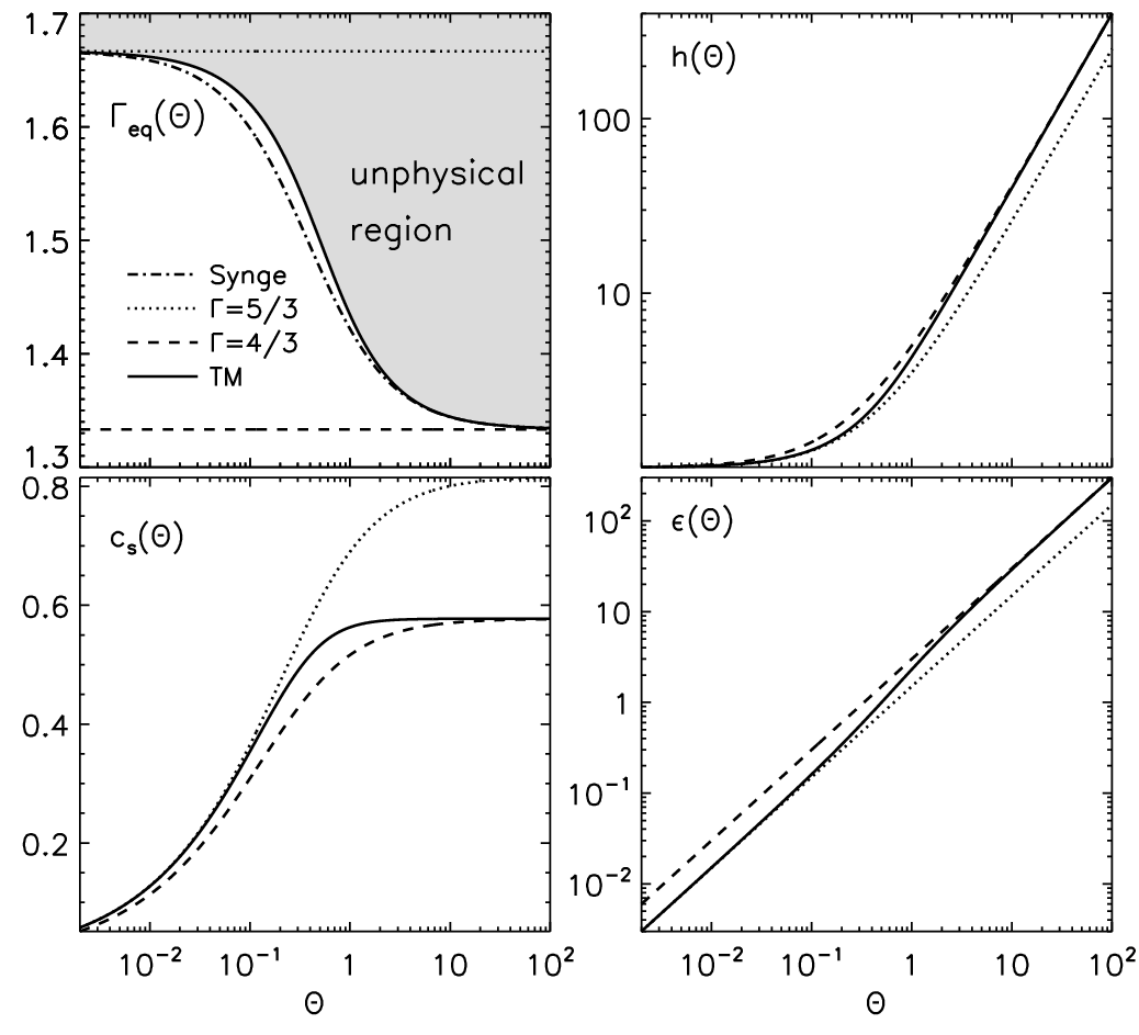
Proper closure to the conservation law (1) is required in order to solve the equations. This is achieved by specifying an EoS relating thermodynamic quantities. The theory of relativistic perfect gases shows that the specific enthalpy is a function of the temperature alone and it takes the form (Synge 1957)
| (9) |
where and are, respectively, the order 2 and 3 modified Bessel functions of the second kind. Equation (9) holds for a gas composed of material particles with the same mass and in the limit of small free path when compared to the sound wavelength.
Direct use of Eq. (9) in numerical codes, however, results in time-consuming algorithms and alternative approaches are usually sought. The most widely used and popular one relies on the choice of the constant -law EoS
| (10) |
where is the constant specific heat ratio. However, Taub 1948 showed that consistency with the relativistic kinetic theory requires the specific enthalpy to satisfy
| (11) |
known as Taub’s fundamental inequality. Clearly the constant -law EoS does not fulfill (11) for an arbitrary choice of , while (9) certainly does. This is better understood in terms of an equivalent , conveniently defined as
| (12) |
and plotted in the top left panel of Fig. 1 for different EoS. In the limit of low and high temperatures, the physically admissible region is delimited, respectively, by (for ) and (for ). Indeed, Taub’s inequality is always fulfilled when while it cannot be satisfied for for any positive value of the temperature.
In a recent paper, Mignone et al. 2005a showed that if the equal sign is taken in Eq. (11), an equation with the correct limiting values may be derived. The resulting EoS ( henceforth), previously introduced by Mathews 1971, can be solved for the enthalpy, yielding
| (13) |
or, using in (11) with the equal sign,
| (14) |
Direct evaluation of using (13) shows that the EoS differs by less than from the theoretical value given by the relativistic perfect gas EoS (9). The proposed EoS behaves closely to the law in the limit of high temperatures, whereas reduces to the law in the cold gas limit. For intermediate temperatures, thermodynamical quantities (such as specific internal energy, enthalpy and sound speed) smoothly vary between the two limiting cases, as illustrated in Fig. 1. In this respect, Eq. (13) greatly improves over the constant -law EoS and, at the same time, offers ease of implementation over Eq. (9). Since thermodynamics is frequently invoked during the numerical solution of (1), it is expected that direct implementation of Eq. (13) in numerical codes will result in faster and more efficient algorithms.
Thermodynamical quantities such as sound speed and entropy are computed from the law of thermodynamics,
| (15) |
where is the entropy. From the definition of the sound speed,
| (16) |
and using (at constant ), one finds the useful expression
| (17) |
where we set . In a similar way, direct integration of (15) yields with
| (18) |
with given by (13).
3 Propagation of Fast Magneto-sonic Shocks
Motivated by the previous results, we now investigate the role of the EoS on the propagation of magneto-sonic shock waves. To this end, we proceed by constructing a one-parameter family of shock waves with different velocities, traveling in the positive direction. States ahead and behind the front are labeled with and , respectively, and are related by the jump conditions
| (19) |
where is the shock speed and is the jump across the wave for any quantity . The set of jump conditions (19) may be reduced (Lichnerowicz 1976) to the following five positive-definite scalar invariants
| (20) |
| (21) |
| (22) |
| (23) |
| (24) |
where
| (25) |
is the mass flux across the shock, and
| (26) |
Here denotes the Lorentz factor of the shock. Fast or slow magneto-sonic shocks may be discriminated through the condition (for the formers) or (for the latters), where .
We consider a pre-shock state characterized by a cold () gas with density . Without loss of generality, we choose a frame of reference where the pre-shock velocity normal to the front vanishes, i.e., . Notice that, for a given shock speed, can be computed from the pre-shock state and thus one has to solve only Eqns. (21)–(24).
3.1 Purely Hydrodynamical Shocks

In the limit of vanishing magnetic field, only Eqns. (23) and (24) need to be solved. Since is given, the problem simplifies to the nonlinear system of equations
| (27) | |||||
| (28) |
We solve the previous equations starting from , for which we were able to provide a sufficiently close guess to the downstream state. Once the and have been found, we repeat the process by slowly increasing the shock velocity and using the previously converged solution as the initial guess for the new value of .
Fig. 2 shows the compression ratio, post-shock internal energy and Mach number as functions of the shock four velocity . For weakly relativistic shock speeds and vanishing tangential velocities (left panels), density and pressure jumps approach the classical (i.e. non relativistic) strong shock limit at , with the density ratio being or depending on the value of ( or , respectively). The post-shock temperature keeps non-relativistic values () and the TM EoS behaves closely to the case, as expected.
With increasing shock velocity, the compression ratio does not saturate to a limiting value (as in the classical case) but keeps growing at approximately the same rate for the constant -law EoS cases, and more rapidly for the TM EoS. This can be better understood by solving the jump conditions in a frame of reference moving with the shocked material and then transforming back to our original system. Since thermodynamics quantities are invariant one finds that, in the limit , the internal energy becomes and the compression ratio takes the asymptotic value
| (29) |
when the ideal EoS is adopted. Since can take arbitrarily large values, the downstream density keeps growing indefinitely. At the same time, internal energy behind the shock rises faster than the rest-mass energy, eventually leading to a thermodynamically relativistic configuration. In absence of tangential velocities (left panels in Fig. 2), this transition starts at moderately high shock velocities () and culminates when the shocked gas heats up to relativistic temperatures () for . In this regime the TM EoS departs from the case and merges on the curve. For very large shock speeds, the Mach number tends to the asymptotic value , regardless of the frame of reference.
Inclusion of tangential velocities (right panels in Fig. 2) leads to an increased mass flux () and, consequently, to higher post-shock pressure and density values. Still, since pressure grows faster than density, temperature in the post-shock flow strains to relativistic values even for slower shock velocities and the TM EoS tends to the case at even smaller shock velocities ().
Generally speaking, at a given shock velocity, density and pressure in the shocked gas attain higher values for lower . Downstream temperature, on the other hand, follows the opposite trend being higher as and lower when .
3.2 Magnetized Shocks


In presence of magnetic fields, we solve the nonlinear system given by Eqns. (22), (23) and (24), and directly replace with the aid of Eq. (21). The magnetic field introduces three additional parameters, namely, the thermal to magnetic pressure ratio () and the orientation of the magnetic field with respect to the shock front and to the tangential velocity. This is expressed by the angles and such that , , . We restrict our attention to the case of a strongly magnetized pre-shock flow with .
Fig. 3 shows the density, plasma and magnetic pressure ratios versus shock velocity for (left panels) and (perpendicular shock, right panels). Since there is no tangential velocity, the solution depends on one angle only () and the choice of is irrelevant. For small shock velocities (), the front is magnetically driven with density and pressure jumps attaining lower values than the non-magnetized counterpart. A similar behavior is found in classical MHD (Jeffrey & Taniuti 1964). Density and magnetic compression ratios across the shock reach the classical values around (rather than as in the non-magnetic case) and increase afterwards. The magnetic pressure ratio grows faster for the perpendicular shock, whereas internal energy and density show little dependence on the orientation angle . As expected, the TM EoS mimics the constant case at small shock velocities. At , the plasma exceeds unity and the shock starts to be pressure-dominated. In other words, thermal pressure eventually overwhelms the Lorentz force and the shock becomes pressure-driven for velocities of the order of . When , the internal energy begins to become comparable to the rest mass energy () and the behavior of the TM EoS detaches from the curve and slowly joins the case. The full transition happens in the limit of strongly relativistic shock speeds, .
Inclusion of transverse velocities in the right state affects the solution in a way similar to the non-magnetic case. Relativistic effects play a role already at small velocities because of the increased inertia of the pre-shock state introduced by the upstream Lorentz factor. For (Fig. 4), the compression ratio does not drop to small values and keeps growing becoming even larger () than the previous case when . The same behavior is reflected on the growth of magnetic pressure that, in addition, shows more dependence on the relative orientation of the velocity and magnetic field projections in the plane of the front. When , indeed, magnetic pressure attains very large values (, bottom right panel in Fig. 4). Consequently, this is reflected in a decreased post-shock plasma . For the TM EoS, the post-shock properties of the flow begin to resemble the behavior at lower shock velocities than before, . Similar considerations may be done for the case of a perpendicular shock (, see Fig. 5), although the plasma saturates to larger values thus indicating larger post-shock pressures. Again, the maximum increase in magnetic pressure occurs when the velocity and magnetic field are perpendicular.
4 Numerical Simulations
With the exception of very simple flow configurations, the solution of the RMHD fluid equations must be carried out numerically. This allows an investigation of highly nonlinear regimes and complex interactions between multiple waves. We present some examples of astrophysical relevance, such as the propagation of one dimensional blast waves, the propagation of axisymmetric jets, and the evolution of magnetized accretion disks around Kerr black holes. Our goal is to outline the qualitative effects of varying the EoS for some interesting astrophysical problems rather than giving detailed results on any individual topic.
Direct numerical integration of Eq. (1) has been achieved using the PLUTO code (Mignone et al. 2007) in §4.1, §4.2 and HARM (Gammie et al. 2003) in §4.3. The new primitive variable inversion scheme presented in Appendix A has been implemented in both codes and the results presented in §4.1 were used for code validation. The novel inversion scheme offers the advantage of being suitable for a more general EoS and avoiding catastrophic cancellation in the non-relativistic and ultrarelativistic limits.
4.1 Relativistic Blast Waves


A shock tube consists of a sharp discontinuity separating two constant states. In what follows we will be considering the one dimensional interval with a discontinuity placed at . For the first test problem, states to the left and to the right of the discontinuity are given by for the left state and for the right state. This results in a mildly relativistic configuration yielding a maximum Lorentz factor of . The second test consists of a left state given by and a right state . This configuration involves the propagation of a stronger blast wave yielding a more relativistic configuration (). For both states, we use a base grid with zones and levels of refinement (equiv. resolution = ) and evolve the solution up to .
Computations carried with the ideal EoS with and the TM EoS are shown in Fig. 6 and Fig. 7 for the first and second shock tube, respectively. From left to right, the wave pattern is comprised of a fast and slow rarefactions, a contact discontinuity and a slow and a fast shocks. No rotational discontinuity is observed. Compared to the case, one can see that the results obtained with the TM EoS show considerable differences. Indeed, waves propagate at rather smaller velocities and this is evident at the head and the tail points of the left-going magneto-sonic rarefaction waves. From a simple analogy with the hydrodynamic counterpart, in fact, we know that these points propagate increasingly faster with higher sound speed. Since the sound speed ratio of the TM and is always less than one (see, for instance, the bottom left panel in Fig. 1), one may reasonably predict slower propagation speed for the Riemann fans when the TM EoS is used. Furthermore, this is confirmed by computations carried with that shows even slower velocities. Similar conclusions can be drawn for the shock velocities. The reason is that the opening of the Riemann fan of the TM equation state is smaller than the case, because the latter always over-estimates the sound speed. The higher density peak behind the slow shock follows from the previous considerations and the conservation of mass across the front.
4.2 Propagation of Relativistic Jets


Relativistic, pressure-matched jets are usually set up by injecting a supersonic cylindrical beam with radius into a uniform static ambient medium (Martí et al. 1997, see, for instance,). The dynamical and morphological properties of the jet and its interaction with the surrounding are most commonly investigated by adopting a three parameter set: the beam Lorentz factor , Mach number and the beam to ambient density ratio . The presence of a constant poloidal magnetic field introduces a fourth parameter , which specifies the thermal to magnetic pressure ratio.
4.2.1 One Dimensional Models
The propagation of the jet itself takes place at the velocity , defined as the speed of the working surface that separates shocked ambient fluid from the beam material. A one-dimensional estimate of (for vanishing magnetic fields) can be derived from momentum flux balance in the frame of the working surface (Martí et al. 1997). This yields
| (30) |
where and are the specific enthalpies of the beam and the ambient medium, respectively. For given and density contrast , Eq. (30) may be regarded as a function of the Mach number alone that uniquely specifies the pressure through the definitions of the sound speed, Eq. (17). For the constant -law EoS the inversion is straightforward, whereas for the TM EoS one finds, using the substitution ,
| (31) |
where satisfies the negative branch of the quadratic equation
| (32) |
with . In Fig. 8 we show the jet velocity for increasing Mach numbers (or equivalently, decreasing sound speeds) and different density ratios . The Lorentz beam factor is . Prominent discrepancies between the selected EoS arise at low Mach numbers, where the relative variations of the jet speed between the constant and the TM EoS’s can be more than . This regime corresponds to the case of a hot jet ( in the case) propagating into a cold () medium, for which neither the nor the approximation can properly characterize both fluids.
4.2.2 Two Dimensional Models
Of course, Eq. (30) is strictly valid for one-dimensional flows and the question remains as to whether similar conclusions can be drawn in more than one dimension. To this end we investigate, through numerical simulations, the propagation of relativistic jets in cylindrical axisymmetric coordinates . We consider two models corresponding to different sets of parameters and adopt the same computational domain (in units of jet radius) with the beam being injected at the inlet region (, ). Jets are in pressure equilibrium with the environment.
In the first model, the density ratio, beam Lorentz factor and Mach number are given, respectively, by , and . Magnetic fields are absent. Integration are carried at the resolution of zones per beam radius using the relativistic Godunov scheme described in MPB. Computed results showing density and internal energy maps at are given in Fig. 9 for , and the TM EoS. The three different cases differ in several morphological aspects, the most prominent one being the position of the leading bow shock, when , for and for the TM EoS. Smaller values of lead to larger beam internal energies and therefore to an increased momentum flux, in agreement with the one dimensional estimate (30). This favors higher propagation velocities and it is better quantified in Fig. 10 where the position of the working surface is plotted as a function of time and compared with the one dimensional estimate. For the cold jet (), the Mach shock exhibits a larger cross section and is located farther behind the bow shock when compared to the other two models. As a result, the jet velocity further decreases promoting the formation of a thicker cocoon. On the contrary, the hot jet () propagates at the highest velocity and the cocoon has a more elongated shape. The beam propagates almost undisturbed and cross-shocks are weak. Close to is termination point, the beam widens and the jet slows down with hot shocked gas being pushed into the surrounding cocoon at a higher rate. Integration with the TM EoS reveals morphological and dynamical properties more similar to the case, although the jet is slower. At the beam does not seem to decelerate and its speed remains closer to the one-dimensional expectation. The cocoon develops a thinner structure with a more elongated conical shape and cross shocks form in the beam closer to the Mach disk.
In the second case, we compare models C2-pol-1 and B1-pol-1 of Leismann et al. 2005 (corresponding to an ideal gas with and , respectively) with the TM EoS adopting the same numerical scheme. For this model, , , and the ambient medium is threaded by a constant vertical magnetic field, . Fig. 11 shows the results at and , corresponding to the final integration times shown in Leismann et al. 2005 for the selected values of . For the sake of conciseness, integration pertaining to the TM EoS only are shown and the reader is reminded to the original work by Leismann et al. 2005 for a comprehensive description. Compared to ideal EoS cases, the jet shown here possesses morphological and dynamical properties intermediate between the hot () and the cold () cases. As expected, the jet propagates slower than in model B1-pol-1 (hot jet), but faster than the cold one (C2-pol-1). The head of the jet tends to form a hammer-like structure (although less prominent than the cold case) towards the end of the integration, i.e., for , but the cone remains more confined at previous times. Consistently with model C2-pol-1, the beam develops a series of weak cross shocks and outgoing waves triggered by the interaction of the flow with bent magnetic field lines. Although the magnetic field inhibits the formation of eddies, turbulent behavior is still observed in cocoon, where interior cavities with low magnetic fields are formed. In this respect, the jet seems to share more features with the cold case.
4.3 Magnetized Accretion near Kerr Black Holes


In this section we study time-dependent GRMHD numerical models of black hole accretion in order to determine the effect of the EoS on the behavior of the accretion disk, corona, and jet. We study three models similar to the models studied by McKinney & Gammie 2004 for a Kerr black hole with and a disk with a scale height () to radius () ratio of . The constant -law EoS with and the TM EoS are used. The initial torus solution is in hydrostatic equilibrium for the -law EoS, but we use the EoS as an initial condition for the TM EoS. Using the EoS as an initial condition for the TM EoS did not affect the final quasi-stationary behavior of the flow. The simplest question to ask is which value of will result in a solution most similar to the TM EoS model’s solution.
More advanced questions involve how the structure of the accretion flow depends on the EoS. The previous results of this paper indicate that the corona above the disk seen in the simulations (De Villiers et al. 2003; McKinney & Gammie 2004) will be most sensitive to the EoS since this region can involve both non-relativistic and relativistic temperatures. The corona is directly involved is the production of a turbulent, magnetized, thermal disk wind (McKinney & Narayan 2006a; McKinney & Narayan 2006b), so the disk wind is also expected to depend on the EoS. The disk inflow near the black hole has a magnetic pressure comparable to the gas pressure (McKinney & Gammie 2004), so the EoS may play a role here and affect the flux of mass, energy, and angular momentum into the black hole. The magnetized jet associated with the Blandford & Znajek 1977 solution seen in simulations (McKinney & Gammie 2004; McKinney 2006) is not expected to depend directly on the EoS, but may depend indirectly through the confining action of the corona. Finally, the type of field geometries observed in simulations that thread the disk and corona (Hirose et al. 2004; McKinney 2005) might depend on the EoS through the effect of the stiffness (larger leads to harder EoSs) of the EoS on the turbulent diffusion of magnetic fields.
Figs. 12, 13 and 14 show a snapshot of the accretion disk, corona, and jet at . Overall the results are quite comparable, as could be predicted since the models studied in McKinney & Gammie 2004 were quite similar. For all models, the field geometries allowed are similar to that found in McKinney 2005. The accretion rate of mass, specific energy, and specific angular momentum are similar for all models, so the EoS appears to have only a small effect on the flow through the disk near the black hole.
The most pronounced effect is that the soft EoS () model develops more vigorous turbulence due to the non-linear behavior of the magneto-rotational instability (MRI) than either the or TM EoSs. This causes the coronae in the model to be slightly thicker and to slightly more strongly confine the magnetized jet resulting in a slight decrease in the opening angle of the magnetized jet at large radii. Also, the model develops a fast magnetized jet at slightly smaller radii than the other models. An important consequence is that the jet opening angle at large radii might depend sensitively on the EoS of the material in the accretion disc corona. This should be studied in future work.
5 Conclusions
The role of the EoS in relativistic magnetohydrodynamics has been investigated both analytically and numerically. The equation of state previously introduced by Mignone et al. 2005a (for non magnetized flows) has been extended to the case where magnetic fields are present. The proposed equation of state closely approximates the single-specie perfect relativistic gas, but it offers a much simpler analytical representation. In the limit of very large or very small temperatures, for instance, the equivalent specific heat ratio reduces, respectively, to the or limits.
The propagation of fast magneto-sonic shock waves has been investigated by comparing the constant laws to the new equation of state. Although for small shock velocities the shock dynamics is well described by the cold gas limit, dynamical and thermodynamical quantities (such as the compression ratio, internal energy, magnetization and so forth) substantially change across the wave front at moderately or highly relativistic speeds. Eventually, for increasing shock velocities, flow quantities in the downstream region smoothly vary from the cold () to the hot () regimes.
We numerically studied the effect of the EoS on shocks, blast waves, the propagation of relativistic jets, and magnetized accretion flows around Kerr black holes. Our results should serve as a useful guide for future more specific studies of each topic. For these numerical studies, we formulated the inversion from conservative quantities to primitive quantities that allows a general EoS and avoids catastrophic numerical cancellation in the non-relativistic and ultrarelativistic limits. The analytical and numerical models confirm the general result that large temperature gradients cannot be properly described by a polytropic EoS with constant specific heat ratio. Indeed, when compared to a more realistic EoS, for which the polytropic index is a function of the temperature, considerable dynamical differences arises. This has been repeatedly shown in presence of strong discontinuities, such shocks, across which the internal energy can change by several order of magnitude.
We also showed that the turbulent behavior of magnetized accretion flows around Kerr black holes depends on the EoS. The EoS leads to more vigorous turbulence than the or TM EoSs. This affects the thickness of the corona that confines the magnetized jet. Any study of turbulence within the accretion disk, the subsequent generation of heat in the coronae, and the opening and acceleration of the jet (especially at large radii where the cumulative differences due to the EoS in the disc are largest) should use an accurate EoS. The effect of the EoS on the jet opening angle and Lorentz factor at large radii is a topic of future study.
The proposed equation state holds in the limit where effects due to radiation pressure, electron degeneracies and neutrino physics can be neglected. It also omits potentially crucial physical aspects related to kinetic processes (such as suprathermal particle distributions, cosmic rays), plasma composition, turbulence effects at the sub-grid levels, etc. These are very likely to alter the equation of state by effectively changing the adiabatic index computed on merely thermodynamic arguments. Future efforts should properly address additional physical issues and consider more general equations of state.
Acknowledgments
We are grateful to our referee, P. Hughes, for his worthy considerations and comments that led to the final form of this paper. JCM was supported by a Harvard CfA Institute for Theory and Computation fellowship. AM would like to thank S. Massaglia and G. Bodo for useful discussions on the jet propagation and morphology.
References
- Aloy et al. (1999) Aloy, M. A., Ibáñez, J. M. , Martí, J. M. , Gómez, J.-L., Müller, E. 1999, ApJL, 523, L125
- Aloy et al. (1999) Aloy, M. A., Ibáñez, J. M., Martí, J. M., Müller, E. 1999, ApJS, 122, 151
- Anile & Pennisi (1987) Anile, M., & Pennisi, S. 1987, Ann. Inst. Henri Poincaré, 46, 127
- Anile (1989) Anile, A. M. 1989, Relativistic Fluids and Magneto-fluids (Cambridge: Cambridge University Press), 55
- Begelman et al. (1984) Begelman, M. C., Blandford, R. D., & Rees, M. J. 1984, Reviews of Modern Physics, 56, 255
- Bernstein & Hughes (2006) Bernstein, J.P., & Hughers, P.A. 2006, astro-ph/0606012
- Blandford & Znajek (1977) Blandford R. D., Znajek R. L., 1977, MNRAS, 179, 433
- Einfeldt et al. (1991) Einfeldt, B., Munz, C.D., Roe, P.L., and Sjögreen, B. 1991, J. Comput. Phys., 92, 273
- Del Zanna et al. (2003) Del Zanna, L., Bucciantini, N., & Londrillo, P. 2003, Astronomy & Astrophysics, 400, 397 (dZBL)
- De Villiers et al. (2003) De Villiers J.-P., Hawley J. F., Krolik J. H., 2003, ApJ, 599, 1238
- Di Matteo et al. (2002) Di Matteo, T., Perna, R., & Narayan, R. 2002, ApJ, 579, 706
- Duncan & Hughes (1994) Duncan, G. C., & Hughes, P. A. 1994, ApJL, 436, L119
- Duncan et al. (1996) Duncan, C., Hughes, P., & Opperman, J. 1996, ASP Conf. Ser. 100: Energy Transport in Radio Galaxies and Quasars, 100, 143
- Falle & Komissarov (1996) Falle, S. A. E. G., & Komissarov, S. S. 1996, mnras, 278, 586
- Gammie et al. (2003) Gammie, C. F., McKinney, J. C., & Tóth, G. 2003, ApJ, 589, 444
- Giacomazzo & Rezzolla (2005) Giacomazzo, B., & Rezzolla, L. 2005, J. Fluid Mech., xxx
- Hardee et al. (1998) Hardee, P. E., Rosen, A., Hughes, P. A., & Duncan, G. C. 1998, ApJ, 500, 599
- Harten et al. (1983) Harten, A., Lax, P.D., and van Leer, B. 1983, SIAM Review, 25(1):35,61
- Hirose et al. (2004) Hirose S., Krolik J. H., De Villiers J.-P., Hawley J. F., 2004, ApJ, 606, 1083
- Jeffrey & Taniuti (1964) Jeffrey A., Taniuti T., 1964, Non-linear wave propagation. Academic Press, New York
- Kohri & Mineshige (2002) Kohri, K., & Mineshige, S. 2002, ApJ, 577, 311
- Kohri et al. (2005) Kohri, K., Narayan, R., & Piran, T. 2005, ApJ, 629, 341
- Koide (1997) Koide, S. 1997, ApJ, 478, 66
- Komissarov (1997) Komissarov, S. S. 1997, Phys. Lett. A, 232, 435
- Komissarov (1999) Komissarov, S. S. 1999, mnras, 308, 1069
- Leismann et al. (2005) Leismann, T., Antón, L., Aloy, M. A., Müller, E., Martí, J. M., Miralles, J. A., & Ibáñez, J. M. 2005, Astronomy & Astrophysics, 436, 503
- Lichnerowicz (1976) Lichnerowicz, A. 1976, Journal of Mathematical Physics, 17, 2135
- Martí & Müller (2003) Martí, J. M. & Müller, E. 2003, Living Reviews in Relativity, 6, 7
- Martí et al. (1997) Martí, J. M. A., Müller, E., Font, J. A., Ibáñez, J. M. A., & Marquina, A. 1997, ApJ, 479, 151
- Mathews (1971) Mathews, W. G. 1971, ApJ, 165, 147
- Meier et al. (2001) Meier, D. L., Koide, S., & Uchida, Y. 2001, Science, 291, 84
- Meliani et al. (2004) Meliani, Z., Sauty, C., Tsinganos, K., & Vlahakis, N. 2004, Astronomy & Astrophysics, 425, 773
- McKinney & Gammie (2004) McKinney, J. C., & Gammie, C. F. 2004, ApJ, 611, 977
- McKinney (2005) McKinney, J. C. 2005, ApJL, 630, L5
- McKinney (2006) McKinney, J. C. 2006, MNRAS, 368, 1561
- McKinney & Narayan (2006a) McKinney J. C., Narayan R., 2006a, MNRAS, in press (astro-ph/0607575)
- McKinney & Narayan (2006b) McKinney J. C., Narayan R., 2006b, MNRAS, in press (astro-ph/0607576)
- Mignone et al. (2005a) Mignone, A., Plewa, T., and Bodo, G. 2005, ApJS, 160, 199
- Mignone et al. (2005) Mignone, A., Massaglia, S., & Bodo, G. 2005, Space Science Reviews, 121, 21
- Mignone & Bodo (2006) Mignone, A., & Bodo, G. 2006, MNRAS, 368, 1040
- Mignone et al. (2007) Mignone, A., Bodo, G., Massaglia, S., Matsakos, T., Tesileanu, O., Zanni, C., and A. Ferrari 2006, accepted for publication on ApJ.
- Misner et al. (1973) Misner, C. W., Thorne, K. S., & Wheeler, J. A. 1973, Gravitation, San Francisco: W.H. Freeman and Co., 1973
- Mizuta et al. (2004) Mizuta, A., Yamada, S., & Takabe, H. 2004, ApJ, 606, 804
- Nishikawa et al. (1997) Nishikawa, K.-I., Koide, S., Sakai, J.-I., Christodoulou, D. M., Sol, H., & Mutel, R. L. 1997, ApJL, 483, L45
- Noble et al. (2006) Noble, S. C., Gammie, C. F., McKinney, J. C., & Del Zanna, L. 2006, ApJ, 641, 626
- Popham et al. (1999) Popham, R., Woosley, S. E., & Fryer, C. 1999, ÀpJ, 518, 356
- Ryu et al. (2006) Ryu, D., Chattopadhyay, I., & Choi, E. 2006, ApJS, 166, 410
- Scheck et al. (2002) Scheck, L., Aloy, M. A., Martí, J. M., Gómez, J. L., Müller, E. 2002, MNRAS, 331, 615
- Synge (1957) Synge, J. L. 1957, The relativistic Gas, North-Holland Publishing Company
- Taub (1948) Taub, A. H. 1948, Physical Review, 74, 328
- Tchekhovskoy et al. (2006) Tchekhovskoy, A, McKinney, J. C.,& Narayan, R. 2006, MNRAS, submitted
- Toro (1997) Toro, E. F. 1997, Riemann Solvers and Numerical Methods for Fluid Dynamics, Springer-Verlag, Berlin
- van Putten (1993) van Putten, M. H. P. M. 1993, ApJL, 408, L21
Appendix A Primitive Variable Inversion Scheme
We outline a new primitive variable inversion scheme that is used to convert the evolved conserved quantities into so-called primitive quantities that are necessary to obtain the fluxes used for the evolution. This scheme allows a general EoS by only requiring specification of thermodynamical quantities and it also avoids catastrophic cancellation in the non-relativistic and ultrarelativistic limits. Large Lorentz factors (up to ) may not be uncommon in some astrophysical contexts (e.g. Gamma-Ray-Burst) and ordinary inversion methods can lead to severe numerical problems such as effectively dividing by zero and subtractive cancellation, see, for instance, Bernstein & Hughes 2006.
First, we note that the general relativistic conservative quantities can be written more like special relativistic quantities by choosing a special frame in which to measure all quantities. A useful frame is the zero angular momentum (ZAMO) observer in an axisymmetric space-time. See Noble et al. 2006 for details. From their expressions, it is useful to note that catastrophic cancellations for non-relativistic velocities can be avoided by replacing in any expression with , where here is the relative 4-velocity in the ZAMO frame. From here on the expressions are in the ZAMO frame and appear similar to the same expressions in special relativity.
A.1 Inversion Procedure
Numerical integration of the conservation law (1) proceeds by evolving the conservative state vector in time. Computation of the fluxes, however, requires velocity and pressure to be recovered from by inverting Eqns. (5)–(7), a rather time consuming and challenging task. For the constant- law, a recent work by Noble et al. 2006 examines several methods of inversion. In this section we discuss how to modify the equations of motion, intermediate calculations, and the inversion from conservative to primitive quantities so that the RMHD method 1) permits a general EoS; and 2) avoids catastrophic cancellations in the non-relativistic and ultrarelativistic limits.
Our starting relations are the total energy density (7),
| (33) |
and the square modulus of Eq. (6),
| (34) |
where and . Note that in order for this expression to be accurate in the non-relativistic limit, one should analytically cancel any appearance of in this expression. Eq. (34) can be inverted to express the square of the velocity in terms of the only unknown :
| (35) |
After inserting (35) into (33) one has:
| (36) |
In order to avoid numerical errors in the non-relativistic limit one must modify the equations of motion and several intermediate calculations. One solves the conservation equations with the mass density subtracted from the energy by defining a new conserved quantity () and similarly for the energy flux. In addition, operations based upon can lead to catastrophic cancellations since the residual is often requested and is dominant in the non-relativistic limit. A more natural quantity to consider is or . Also, in the ultrarelativistic limit calculations based upon have catastrophic cancellation errors when . This can be avoided by 1) using instead and 2) introducing the quantities and , with properly rewritten as
| (37) |
to avoid machine accuracy problems in the nonrelativistic limit, where . Thus our relevant equations become:
| (38) |
| (39) |
where .
Equations (38) and (39) may be inverted to find , and . A one dimensional inversion scheme is derived by regarding Eq. (38) as a single nonlinear equation in the only unknown and using Eq. (39) to express as a function of . Using Newton’s iterative scheme as our root finder, one needs to compute the derivative
| (40) |
The explicit form of depends on the particular EoS being used. While prior methods in principle allow for a general EoS, one has to re-derive many quantities that involve kinematical expressions. This can be avoided by splitting the kinematical and thermodynamical quantities. This also allows one to write the expressions so that there is no catastrophic cancellations in the non-relativistic or ultrarelativistic limits. Assuming that , we achieve this by applying the chain rule to the pressure derivative:
| (41) |
Partial derivatives involving purely thermodynamical quantities must now be supplied by the EoS routines. Derivatives with respect to , on the other hand, involve purely kinematical terms and do not depend on the choice of the EoS. Relevant expressions needed in our computations are given in the Appendix.
Once has been determined to some accuracy, the inversion process is completed by computing the velocities from an inversion of equation (6) to obtain
| (42) |
One then computes from an inversion of equation (37) to obtain
| (43) |
from which or can be obtained for any given EoS. The rest mass density is obtained from
| (44) |
and the magnetic field is trivially inverted.
In summary, we have formulated an inversion scheme that 1) allows a general EoS without re-deriving kinematical expressions; and 2) avoids catastrophic cancellation in the non-relativistic and ultrarelativistic limits. This inversion involves solving a single non-linear equation using, e.g., a one-dimensional Newton’s method. A similar two-dimensional method can be easily written with the same properties, and such a method may be more robust in some cases since the one-dimensional version described here involves more complicated non-linear expressions.
One can show analytically that the inversion is accurate in the ultrarelativistic limit as long as for and for pressure, where for double precision. The method used by Noble et al. 2006 requires due to the repeated use of the expression in the inversion. Note that we use that has no catastrophic cancellation. The fundamental limit on accuracy is due to evolving energy and momentum separately such that the expression appears in the inversion. Only a method that evolves this quantity directly (e.g. for one-dimensional problems one can evolve the energy with momentum subtracted) can reach higher Lorentz factors. An example test problem is the ultrarelativistic Noh test in Aloy et al. 1999 with , , (i.e. ) This test has , which is just below double precision and so the pressure is barely resolved in the pre-shock region. The post-shock region is insensitive to the pre-shock pressure and so is evolved accurately up to . These facts are have been also confirmed numerically using this inversion within HARM. Using the same error measures as in Aloy et al. 1999 we can evolve their test problem with an even higher Lorentz factor of and obtain similar errors of .
A.2 Kinematical and Thermodynamical Expressions
The kinematical terms required in equation (41) may be easily found from the definition of ,
| (45) |
by straightforward differentiation. This yields
| (46) |
and
| (47) |
where
| (48) |
is computed by differentiating (35) with respect to (note that ). Equation (46) does not depend on the knowledge of the EoS.
Thermodynamical quantities such as , on the other hand, do require the explicit form of the EoS. For the ideal gas EoS one simply has
| (49) |
where . By taking the partial derivatives of (49) with respect to (keeping constant) and (keeping constant) one has
| (50) |
For the TM EoS, one can more conveniently rewrite (14) as
| (51) |
which, upon differentiation with respect to (keeping constant) yields
| (52) |
Similarly, by taking the derivative with respect to at constant gives
| (53) |
In order to use the above expressions and avoid catastrophic cancellation in the non-relativistic limit, one must solve for the gas pressure as functions of only and and then write the pressure that explicitly avoids catastrophic cancellation as . One obtains:
| (54) |
Also, for setting the initial conditions it is useful to be able to convert from a given pressure to the internal energy by using
| (55) |
which also avoids catastrophic cancellation in the non-relativistic limit.
A.3 Newton-Raphson Scheme
Equation (38) may be solved using a Newton-Raphson iterative scheme, where the -th approximation to the is computed as
| (56) |
where
| (57) |
and is given by Eq. (40). The iteration process terminates when the residual falls below some specified tolerance.
We remind the reader that, in order to start the iteration process given by (56), a suitable initial guess must be provided. We address this problem by initializing, at the beginning of the cycle, , where is the positive root of
| (58) |
and is the quadratic function
| (59) |
This choice guarantees positivity of pressure, as it can be proven using the relation
| (60) |
which follows upon eliminating the term in Eq. (34) with the aid of Eq. (33). Seeing that is a convex quadratic function, the condition is equivalent to the requirement that the solution must lie outside the interval , where . However, since , it must follow that and thus lies outside the specified interval. We tacitly assume that the roots are always real, a condition that is always met in practice.