Heisenberg antiferromagnet with anisotropic exchange on the kagomé lattice: Description of the magnetic properties of volborthite

T. Yavors’kii Affiliation: Department of Physics and Astronomy, University of Waterloo, 200 University Avenue W, Waterloo, N2L 3G1, Canada. W. Apel Affiliation: Physikalisch-Technische Bundesanstalt, Bundesallee 100, D-38116 Braunschweig, Germany. H.-U. Everts Affiliation: Institut für Theoretische Physik, Leibniz Universität Hannover, Appelstraße 2, D-30167 Hannover, Germany.

August 11, 2026

Abstract

We study the properties of the Heisenberg antiferromagnet with spatially anisotropic nearest-neighbour exchange couplings on the kagomé net, i.e., with coupling $J$ in one lattice direction and couplings $J^{\prime}$ along the other two directions. For $J/J^{\prime}\gtrsim 1$ , this model is believed to describe the magnetic properties of the mineral volborthite. In the classical limit, it exhibits two kinds of ground states: a ferrimagnetic state for $J/J^{\prime}<1/2$ and a large manifold of canted spin states for $J/J^{\prime}>1/2$ . To include quantum effects self-consistently, we investigate the ${\rm Sp(\mathcal{N})}$ symmetric generalisation of the original ${\rm SU(2)}$ symmetric model in the large- $\mathcal{N}$ limit. In addition to the dependence on the anisotropy, the ${\rm Sp(\mathcal{N})}$ symmetric model depends on a parameter $\kappa$ that measures the importance of quantum effects. Our numerical calculations reveal that in the $\kappa$ - $J/J^{\prime}$ plane, the system shows a rich phase diagram containing a ferrimagnetic phase, an incommensurate phase, and a decoupled chain phase, the latter two with short- and long-range order. We corroborate these results by showing that the boundaries between the various phases and several other features of the ${\rm Sp(\mathcal{N})}$ phase diagram can be determined by analytical calculations. Finally, the application of a block-spin perturbation expansion to the trimerised version of the original spin- $1/2$ model leads us to suggest that in the limit of strong anisotropy, $J/J^{\prime}\gg 1$ , the ground state of the original model is a collinearly ordered antiferromagnet, which is separated from the incommensurate state by a quantum phase transition.

pacs

75.10.Jm,75.30.Kz,75.50.Ee

I Introduction

In the ongoing search for novel states of condensed matter, frustrated antiferromagnets have played a key role (for a recent review, see Ref. Misguich and Lhuillier 2004). Among the many substances that have been investigated experimentally and the numerous spin models that have been studied theoretically, those in which the magnetic ions occupy the vertices of corner-sharing frustrating entities have attracted particular attention in this context. The best known examples are the kagomé antiferromagnet (KAF), consisting of corner sharing triangles, and the pyrochlore antiferromagnet, consisting of corner sharing tetrahedra (see Fig. 1).

Refer to caption — Figure 1: kagomé lattice (a), pyrochlore lattice (b)

The main distinction between the KAF, the pyrochlore antiferromagnet and other frustrated and unfrustrated magnets is the large ground-state degeneracy of the former: classical Heisenberg antiferromagnets with nearest-neighbour interactions on corner-sharing lattices have a large ground-state degeneracy, which in the above two examples even leads to a finite ground-state entropy (see, e.g., Ref. Moessner 2001 and references therein). Quantum effects may lift this degeneracy, and, indeed, in numerical studies of small cells of the spin $\frac{1}{2}$ KAF, an exponentially large number of very low-lying quantum states has been observed Lecheminant et al. 1997; Waldtmann et al. 1998. It has been suggested that this abundance of low-lying states can be understood in a description of the low-energy physics of the quantum KAF as spin liquid consisting of nearest-neighbour spin singlets Mila 1998; Mambrini and Mila 2000. However, a complete picture of the ground state and of the excitations of the KAF is still missing. Further theoretical, but also experimental studies with emphasis on the quantum properties of the KAF are therefore highly desirable. In this last respect, the mineral volborthite is a very promising candidate. It has been the subject of several recent experimental investigations Hiroi et al. 2001; Fukaya et al. 2003; Bert et al. 2004; Bert et al. 2005. The magnetic lattice of this natural antiferromagnet consists of the $S=1/2$ spins of $Cu^{2+}$ ions that are located on the vertices of well separated planar kagomé-like nets. A monoclinic distortion of the lattice leads to a slight difference between the exchange couplings along one lattice direction ( $J$ ) and the two other directions ( $J^{\prime}$ )(see Fig. 2). Since neither signs of long-range order nor signs of a spin-gapped singlet ground-state were found in experiments on volborthite, the substance seems to be a good candidate for the observation of the low-energy features that are thought to be typical for kagomé type antiferromagnets Misguich and Lhuillier 2004.

Whether and to what extent the different exchange couplings along different lattice directions of the kagomé net of volborthite influence the low-energy physics of the system is presently unknown. In the present paper, we study this question on the basis of the model Hamiltonian

\mathcal{H}_{\rm AKAF}=J\sum_{[i,j]}{\mathbf{S}}_{i}{\mathbf{S}}_{j}+J^{\prime}\sum_{\langle k,i\rangle}{\mathbf{S}}_{k}{\mathbf{S}}_{i}\;.

(1)

The symbols $[i,j]$ and $\langle k,i\rangle$ denote, respectively, bonds between nearest-neighbour sites on the horizontal chains ( $a$ , $b$ ) and bonds between the middle sites ( $c$ ) and the sites $a$ , $b$ , see Fig. 2. Since the physics of this model depends only on the ratio $J/J^{\prime}$ of the exchange constants, we set $J^{\prime}=1$ in the sequel. We will consider the spatially anisotropic kagomé antiferromagnet (AKAF), Eq. (1), in the full range of $J$ , $0<J<\infty$ since this is of theoretical interest: one expects to see quantum phase transitions as $J$ is increased. It is of particular interest to find out whether there is a transition from two-dimensional magnetic states to a set of decoupled chains with free spins on the axes between the chains for large values of $J$ .

The paper is organised as follows. In Sec. II, we consider the model (1) in the classical limit. At this level, we find no sign of a transition from the two-dimensional magnet to a set of decoupled chains as $J$ increases to infinity. Nonetheless, the ground-state degeneracy, as well as the spin wave spectrum are found to change qualitatively as the anisotropy of the model varies. In Sec. III, we consider a generalisation of the ${\rm SU(2)}$ symmetric model (1) to the ${\rm Sp(\mathcal{N})}$ symmetric version Sachdev and Read 1991; Sachdev 1992 and describe its properties in the large- $\mathcal{N}$ limit, where a mean-field treatment of the model is adequate. We obtain a detailed description of how possible ground states of the model depend on the coupling $J$ and on the spin length $S$ . A fairly rich phase diagram with a ferrimagnetic phase for small $J$ , long-range ordered and short-ranged incommensurate phases for intermediate values of $J$ , and a decoupled-chain phase for large $J$ emerges. Parts of these results have been published previously, see Ref. Apel et al. 2007. In Sec. IV, we devise trial quantum ground states of the original $S=1/2$ model. We chose the states such that they are exact eigenstates of $\mathcal{H}_{\rm AKAF}$ , if the couplings on the upward pointing triangles of Fig. 2 are switched off, and we then treat these couplings perturbatively. In the limit $J\longrightarrow\infty$ this yields an effective Hamiltonian for the spins on the $c$ sites which represents an anisotropic triangular antiferromagnet. The conclusions of Starykh and Balents Starykh and Balents 2007 about the ground state of this effective model lead us to conjecture the existence of a quantum phase transition in the AKAF for large $J$ . In Sec. V, we summarise and discuss our results. In two Appendices, we present technical details of the counting procedure for the classical ground-states, and of the Ginzburg-Landau type procedure that allows us to determine the boundaries in the phase diagram analytically.

II Classical and semiclassical aspects

Similar to other isotropic spin models on lattices with triangular elementary cells, the classical ground states of $\mathcal{H}_{\rm AKAF}$ , Eq. (1), are spin configurations, which satisfy the condition that for each elementary triangular plaquette of the lattice, Fig. 2, the energy is minimal.

For $J=0$ , this yields a ferrimagnetic state with the chain spins aligned in one direction and the middle spins pointing in the opposite direction, so that the total magnetisation is $M=N_{\bigtriangledown}S$ ( $N_{\bigtriangledown}$ : number of downward pointing triangles, $N_{\bigtriangledown}=N_{s}/3$ where $N_{s}$ is the number of sites of the system). We illustrate this situation in Fig. 3. According to the Lieb-Mattis theorem, the exact quantum ground state (GS) of the model $\mathcal{H}_{\rm AKAF}$ also has total spin $S^{tot}=N_{\bigtriangledown}\,S$ for $J=0$ , see Ref. Lieb and Mattis 1962, i.e., for $J=0$ , the quantum GS is ferrimagnetic too. By continuity, one expects the quantum GS to remain ferrimagnetic for sufficiently small finite $J$ . This will be confirmed by our considerations of the large- $\mathcal{N}$ limit of the ${\rm Sp(\mathcal{N})}$ version of our model (see the analytical and numerical work in Sects. III, III.3 and Appendix B) and by the block spin perturbation approach (Sec. IV). Classically, the ferrimagnetic state remains stable up to $J=1/2$ . The excitation spectrum of the ferrimagnetic state obtained in linear spin-wave (LSW) approximation is shown in Fig. 4.

The analytic expressions for these three frequency surfaces $\omega_{\alpha}({\mathbf{q}})$ , $\alpha=1,2,3$ , are obtained as solutions of a third-order secular equation and are too lengthy to be presented here. However, one can easily assure oneself that the dispersion of the gapless mode is quadratic at the origin. Thus, one has the typical mode structure of a ferrimagnet here with one ferromagnetic mode and two optical modes, see, e.g., Ref. Brehmer et al. 1997. As $J$ increases towards $1/2$ , the ferromagnetic frequency surface looses its dispersion and turns into a plane of zero modes, one zero mode for each wave vector in the magnetic Brillouin zone (BZ), at $J=1/2$ . The gap of the lower optical mode closes at this value of $J$ in the centre of the BZ and the dispersion of this mode becomes linear for small wave vectors as for an antiferromagnetic spin-wave mode.

At $J=1/2$ , the classical GS configuration changes from the unique ferrimagnetic state to an ensemble of degenerate canted coplanar states. These states are characterised by two variables: the angle $\theta$ , which the middle spin of a given triangular plaquette forms with the two chain spins of the same plaquette (see Fig. 5), and the two valued chirality $\chi=\pm 1$ , which denotes the direction in which the spins turn as one moves around the plaquette in the mathematically positive sense.

For $J\geq 1/2$ , the requirement that the energy of any of the elementary triangular plaquettes of the lattice Fig. 2 be minimal is $\theta=\arccos(-1/(2J))$ , ( $\theta>0$ ). The different degenerate canted states arise from different possibilities to assign positive or negative chiralities to the plaquettes of the lattice. We show in the Appendix A that for the general case of $\theta\neq 2\pi/3$ ( $J\neq 1$ ), the number of spin configurations, $N^{aniso}_{GS}$ does not grow exponentially with the number of sites. Rather, $N^{aniso}_{GS}<2^{\alpha\sqrt{N_{\bigtriangledown}}}$ , where $\alpha<3$ . This implies that the ground-state entropy per spin of the classical AKAF vanishes in the thermodynamic limit. In this respect, the anisotropic model differs qualitatively from the isotropic KAF in the classical limit, which has an extensive entropy per spin. In the limit $J\rightarrow 1$ , the anisotropic model approaches the isotropic KAF. Hence, one expects that for the anisotropic model there is an extensive number of low-lying excited states that become degenerate with the GS in the isotropic limit.

As in the case of the isotropic KAF, the spin-wave Hamiltonian is in linear order independent of the particular classical GS that has been chosen as the starting point of the expansion, Ref. Harris et al. 1992. This implies that lowest-order quantum fluctuation do not select one or a group of classical GSs as true GSs, i.e., the possible ordering effects of quantum fluctuations are not captured by the linear spin-wave (LSW) approximation. Figs. 6, 7 show the spin-wave frequency surfaces for $J=0.6$ and for $J=3$ . It is easy to show analytically that, as is illustrated in these figures, the plane of zero frequency modes persists for all values of $J$ greater than $1/2$ . The surfaces for $J<1/2$ and for $J>1/2$ join smoothly at $J=1/2$ . Thus, in the LSW approximation, the transition from the ferrimagnetically ordered state to the canted spin states appears to be of second order. For $J\gg 1$ , the nonzero frequencies gradually loose their dispersion perpendicular to the strong- $J$ direction and take the shape of the spin-wave spectrum of antiferromagnetic chains parallel to this direction. However, no sign of a further transition from the canted spin states to a set of decoupled spin chains is found in this semiclassical approach. In the next section, we will consider the symplectic ${\rm Sp(\mathcal{N})}$ generalisation of the antiferromagnetic model $\mathcal{H}_{\rm AKAF}$ in the large- $\mathcal{N}$ limit. This approach, which was first proposed by Read and Sachdev, Refs. Sachdev and Read 1991; Sachdev 1992, as a method to study frustrated antiferromagnets, has the benefit of including the ordering effects of quantum fluctuations self-consistently. It is of particular interest for spin models with two or more competing exchange couplings in the different lattice directions or over different lattice distances such as the present model, the $J_{1}$ - $J_{2}$ - $J_{3}$ model Sachdev and Read 1991, the Shastry-Sutherland antiferromagnet Chung et al. 2001a and the anisotropic triangular antiferromagnet Chung et al. 2001b. For these models, it has provided an unbiased selection of possible GSs that may or may not be ordered depending on the value of a parameter $\kappa$ , which is connected with the spin length $S$ (see below).

III Mean field ${\rm Sp(\mathcal{N})}$ approach

III.1 Brief review of the method

For a general antiferromagnetic Heisenberg model with a positive interaction matrix $J_{ij}$ ,

\mathcal{H}=\sum_{i>j}J_{ij}\;{\bf S}_{i}\cdot{\bf S}_{j}\,,

(2)

the ${\rm Sp(\mathcal{N})}$ generalisation reads

\mathcal{H}_{{\rm Sp(\mathcal{N})}}=-\sum_{i>j}\frac{J_{ij}}{2\mathcal{N}}(\mathcal{J}^{\alpha\beta}b^{\dagger}_{i\alpha}b^{\dagger}_{j\beta})(\mathcal{J}_{\gamma\delta}b_{i}^{\gamma}b_{j}^{\delta})\,.

(3)

Here,

\mathcal{J}=\left(\begin{array}[]{lll}\mbox{\boldmath{$\varepsilon$}}&&\\ &\mbox{\boldmath{$\varepsilon$}}&\\ &&\ddots\end{array}\right)

(4)

is the $2\mathcal{N}\times 2\mathcal{N}$ generalisation of the $2\times 2$ antisymmetric tensor

\mbox{\boldmath{$\varepsilon$}}=\left(\begin{array}[]{c@{\hspace{1mm}}c}0\hfil\hskip 2.84526pt&+1\\ -1\hfil\hskip 2.84526pt&0\end{array}\right)\,,

(5)

and $b_{i}^{\alpha}$ with $\alpha=1,\dots,2\mathcal{N}$ are the ${\rm Sp(\mathcal{N})}$ boson annihilation operators. (Here and in the sequel, we closely follow the notation of Ref. Sachdev 1992; in particular, summation over repeated upper and lower indices is implied.) Thus, $\mathcal{J}^{\alpha\beta}b^{\dagger}_{i\alpha}b^{\dagger}_{j\beta}$ is the generalisation of the creation operator $\varepsilon^{\alpha\beta}b^{\dagger}_{i\alpha}b^{\dagger}_{j\beta}$ for a singlet on the bond $(i,j)$ . For the special case $\mathcal{N}=1$ , one finds

(\mathcal{J}^{\alpha\beta}b^{\dagger}_{i\alpha}b^{\dagger}_{j\beta})(\mathcal{J}_{\gamma\delta}b_{i}^{\gamma}b_{j}^{\delta})=-2{\mathbf{S}_{i}}\cdot{\mathbf{S}_{j}}+n_{bi}n_{bj}/2+\delta_{ij}n_{bi}\,,

(6)

where

n_{bi}=b^{\dagger}_{i\alpha}b_{i}^{\alpha}

(7)

is the boson number operator at site $i$ and where

{\mathbf{S}_{i}}=b^{\dagger}_{i\alpha}{\mbox{\boldmath{$\tau$}}}^{\alpha}_{\beta}b_{i}^{\beta}/2

(8)

is the usual ${\rm SU(2)}$ spin operator at site $i$ . ( $\tau$ are the Pauli matrices). Then, if one imposes the constraint that the number of bosons is the same for all lattice sites, $n_{bi}\equiv n_{b}$ , the Hamiltonian $\mathcal{H}_{{\rm Sp(1)}}$ is the familiar ${\rm SU(2)}$ invariant antiferromagnetic Heisenberg Hamiltonian (plus some constants) with $n_{b}=2S$ .

In the subsequent exposition, we shall consider a Hamiltonian of the form (3) in the large- $\mathcal{N}$ limit following the strategy of Refs. Sachdev and Read 1991; Sachdev 1992. Depending on the values of the couplings $J_{ij}$ and of $\kappa$ , the GS of $\mathcal{H}_{{\rm Sp(\mathcal{N})}}$ may either break the global ${\rm Sp(\mathcal{N})}$ symmetry and exhibit LRO or it may be ${\rm Sp(\mathcal{N})}$ symmetric with only SRO. Breaking of the ${\rm Sp(\mathcal{N})}$ symmetry will happen through condensation, i.e., by macroscopic occupation of one of the Bose fields $b_{\alpha}$ . To allow for this, we introduce the parametrisation

b_{i}^{m\sigma}=\left(\begin{array}[]{l}\sqrt{\mathcal{N}}x_{i}^{\sigma}\\ \tilde{b}_{i}^{\tilde{m}\sigma}\end{array}\right)

(9)

with $\alpha=(m\sigma)$ , $m=1,\cdots,\mathcal{N}$ , $\tilde{m}=2,\cdots,\mathcal{N}$ and $\sigma=\uparrow,\downarrow$ . The field $x_{i}^{\sigma}$ is proportional to the condensate amplitude, $\langle b_{i}^{m\sigma}\rangle=\sqrt{\mathcal{N}}\;\delta_{1}^{m}\;x_{i}^{\sigma}$ . Aiming at a mean field treatment of the Hamiltonian $\mathcal{H}_{{\rm Sp(\mathcal{N})}}$ , which becomes exact in the large $\mathcal{N}$ limit, we decouple the quartic part by the Hubbard-Stratonovich technique with complex fields $Q_{ij}=-Q_{ji}$ and with Lagrange multipliers $\lambda_{i}$ that enforce the local constraints (7). The variables $Q_{ij}$ which are defined on nearest neighbour bonds of the lattice are expectation values of the bond singlet creation operators in the GS, $Q_{ij}=\langle\sum_{\sigma\sigma^{\prime}}\varepsilon^{\sigma\sigma^{\prime}}b_{i\,m\sigma}^{\dagger}b_{j\,m\sigma^{\prime}}^{\dagger}\rangle$ and are to be determined self-consistently from the mean field type Hamiltonian

\mathcal{H}_{\rm MF}=\sum_{i>j}\left\{\frac{\mathcal{N}}{2}J_{ij}|Q_{ij}|^{2}-\frac{1}{2}J_{ij}\left[Q_{ij}\varepsilon_{\sigma\sigma^{\prime}}\left(\mathcal{N}x_{i}^{\sigma}x_{j}^{\sigma^{\prime}}+\sum_{\tilde{m}}\tilde{b}_{i}^{\tilde{m}\sigma}\tilde{b}_{j}^{\tilde{m}\sigma^{\prime}}\right)+h.c.\right]\right\}+{}\sum_{i}\lambda_{i}\left(\mathcal{N}|x_{i}^{\sigma}|^{2}+\sum_{\tilde{m}}\tilde{b}^{\dagger}_{i\tilde{m}\sigma}\tilde{b}_{i}^{\tilde{m}\sigma}-n_{b}\right)\;.

(10)

The variational ground state energy, $E_{\rm MF}$ , of $\mathcal{H}_{\rm MF}$ in the large- $\mathcal{N}$ limit is obtained by diagonalising the bosonic part of $\mathcal{H}_{\rm MF}$ , integrating over the $2(\mathcal{N}-1)N_{s}$ bosonic fields $\tilde{b}_{i}^{\tilde{m}\sigma}$ in the action associated with $\mathcal{H}_{\rm MF}$ . One obtains:

	$\displaystyle\frac{E_{\rm MF}}{\mathcal{N}}$	$\displaystyle=$	$\displaystyle\sum_{i>j}\left[\frac{1}{2}J_{ij}\|Q_{ij}\|^{2}-\frac{1}{2}J_{ij}\left(Q_{ij}\varepsilon_{\sigma\sigma^{\prime}}x_{i}^{\sigma}x_{j}^{\sigma^{\prime}}+h.c.\right)\right]$		(11)
			$\displaystyle+\sum_{{\mathbf{k}},\mu}\omega_{\mu}({\mathbf{k}};Q,\lambda)+\sum_{i}\lambda_{i}\left(\|x_{i}^{\sigma}\|^{2}-1-\kappa\right)\,.$		(11)

Here $\omega_{\mu}({\mathbf{k}};Q,\lambda)$ are the positive eigenvalues of the bosonic part of $\mathcal{H}_{\rm MF}$ , and $\kappa=n_{b}/\mathcal{N}$ is kept fixed in the limiting procedure Sachdev and Read 1991; Sachdev 1992. The parameter $\kappa$ is a measure for the importance of quantum fluctuations: by varying $\kappa$ from small to large values, one drives the system from the regime dominated by quantum fluctuations to the classical regime, i.e., from the disordered into the ordered region. Finally, the GS is obtained by finding the saddlepoint of $E_{\rm MF}$ in the space of the variables $Q_{ij}$ and $x^{\sigma}_{i}$ subject to the constraints

\partial E_{\rm MF}(Q,\lambda)/\partial\lambda_{i}=0\,.

(12)

In addition to the GS itself, the spin-spin correlation function $G_{ij}=\langle{\mathbf{S}_{i}}\cdot{\mathbf{S}_{j}}\rangle$ in the GS is an important piece of information. In particular, by considering its behaviour in the limit $|i-j|\longrightarrow\infty$ , one can distinguish between LRO and SRO. According to Sachdev Sachdev 1992, to obtain $G_{ij}$ in the ${\rm Sp(\mathcal{N})}$ symmetric approach, the ${\rm SU(2)}$ invariant expression ${\mathbf{S}_{i}}\cdot{\mathbf{S}_{j}}$ must be replaced by the ${\rm Sp(\mathcal{N})}$ invariant expression

\frac{1}{4\mathcal{N}^{2}}(b_{i\alpha}^{\dagger}b_{i}^{\beta}b_{j\beta}^{\dagger}b_{j}^{\alpha}-\mathcal{J}^{\alpha\gamma}\mathcal{J}_{\beta\delta}b_{i\alpha}^{\dagger}b_{i}^{\beta}b_{j\gamma}^{\dagger}b_{j}^{\delta}).

(13)

Within the mean field approach, $G_{ij}$ can then be calculated straightforwardly.

III.2 The anisotropic kagomé antiferromagnet

III.2.1 Choice of mean-field variables

We wish to apply the procedure described above to the AKAF represented by the Hamiltonian (1). To render the problem of finding the eigenvalues $\omega_{\mu}$ in Eq. (10) and of optimising $E_{\rm MF}$ tractable, we have to restrict the number of variables $Q_{ij}$ and $\lambda_{i}$ . We do so by demanding that the mean field Hamiltonian $\mathcal{H}_{\rm MF}$ for the spinon operators $b^{(\dagger)}$ is symmetric under transformations of the projective symmetry group (PSG) that is related to the symmetry group of the spin Hamiltonian $\mathcal{H}_{\rm AKAF}$ (Eq. 1) (see Ref. Wang and Vishwanath 2006). We include two translations, a rotation by $\pi$ and a mirror axis orthogonal to the preferred direction of the exchange constants ( $J$ ). Thus generalising the treatment of Wang and Vishwanath to our model, we find eight mean-field states with different symmetries. Seven of them have flux in the sense of Ref. Tchernyshyov et al. 2006 in various cells of the lattice. Following the arguments in Ref. Tchernyshyov et al. 2006, we exclude all flux-carrying states and end up with the solution (cf. Fig. 8) $P_{1,2,3}=Q_{1,2,3}$ , $Q_{3}=Q_{2}$ , and $\lambda_{b}=\lambda_{a}$ .

In order to check the flux-argument in Ref. Tchernyshyov et al. 2006, we have explicitely studied the solution $P_{1,2,3}=-Q_{1,2,3}$ and found that it is always of higher energy (For $J=1$ , this agrees with the result of Ref. Sachdev 1992).

Thus, the expression Eq. (11) can now be cast into the form

	$\displaystyle\frac{E_{\rm MF}}{\mathcal{N}N_{\bigtriangledown}}\;=\;$		$\displaystyle J\,\|Q_{1}\|^{2}+2\,\|Q_{2}\|^{2}-(2\lambda_{a}+\lambda_{c})(\kappa+1)$		(14)
			$\displaystyle+\frac{1}{N_{\bigtriangledown}}\sum_{{\mathbf{k}},\mu}\omega_{\mu}(\mathbf{k})\left(1+\|{x}_{\mu}(\mathbf{k})\|^{2}\right)\,,$		(14)

where the condensate is written in diagonalized form and $\omega_{\mu}(\mathbf{k})$ are the three positive solutions of

\det\mathbf{\hat{D}}(\omega)=0\,.

(15)

Here,

\mathbf{\hat{D}}(\omega)=\left(\begin{array}[]{c@{\hspace*{3mm}}c}\mathbf{\hat{\Lambda}}-\omega\mathbf{\hat{I}}\hfil\hskip 8.53581pt&\mathbf{\hat{Q}}\\ \mathbf{\hat{Q}^{\dagger}}\hfil\hskip 8.53581pt&\mathbf{\hat{\Lambda}}+\omega\mathbf{\hat{I}}\end{array}\right)\,,

(16)

with

	$\displaystyle\mathbf{\hat{\Lambda}}\,$	$\displaystyle=$	$\displaystyle\,diag(\lambda_{a},\,\lambda_{c},\,\lambda_{a})\,,$		(17)
	$\displaystyle\mathbf{\hat{Q}}\,$	$\displaystyle=$	$\displaystyle\,\left(\begin{array}[]{ccc}0&\tilde{Q}_{2}(\mathbf{k})&-J\tilde{Q}_{1}(-\mathbf{k})\\ -\tilde{Q}_{2}(-\mathbf{k})&0&\tilde{Q}_{3}(\mathbf{k})\\ J\tilde{Q}_{1}(\mathbf{k})&-\tilde{Q}_{3}(-\mathbf{k})&0\end{array}\right)\,,$

\mbox{and}\quad\tilde{Q}_{a}(\mathbf{k})=\frac{1}{2}Q_{a}\left(e^{i{\mbox{\boldmath{\scriptsize$\delta$}}}_{a}\mathbf{k}/2}-e^{-i{\mbox{\boldmath{\scriptsize$\delta$}}}_{a}\mathbf{k}/2}\right)\,,\quad a=1,2,3,

(22)

$\mbox{\boldmath{$\delta$}}_{1,2,3}$ , see Fig. 2.

III.2.2 Technical details of the numerical extremalisation

Determination of the ground state of the AKAF in the considered approximation has been reduced to minimization of the Eq. (14) with respect to two variables $Q_{1}$ and $Q_{2}$ , subject to the Lagrange constraints with respect to two parameters $\lambda_{a}$ and $\lambda_{c}$ . Being apparently trivial, the optimization procedure turns out to be quite involved technically.

First, we find it crucial to consider at least two different chemical potentials. Other than for the spatially isotropic KAF, $J=1$ , we were not able to find a non-trivial solution if we used a single $\lambda$ , $\lambda_{a}=\lambda_{b}=\lambda_{c}$ . If $\lambda_{a}$ and $\lambda_{c}$ are different, $[\mathbf{\hat{\Lambda}},\mathbf{\hat{Q}}]\neq 0$ , the Lagrange multipliers enter the expressions for the frequencies $\omega_{\mu}$ non-trivially, other than in the case of a global uniform chemical potential (cf. Ref. Sachdev 1992). In turn, the Lagrange constraints cannot be satisfied semi-analytically, and require a numerical treatment. Second, we choose to work directly in the thermodynamic limit $N_{s}\rightarrow\infty$ of the model (14) by performing a numerical self-adapting integration over the BZ. In this limit, the singularities can be integrated, and symmetry breaking is signalled by the appearance of a finite value of the condensate amplitude ${x_{\mu}}({\mathbf{k}})$ at a certain wavevector ${\mathbf{k}}={\mathbf{q}}_{ord}$ , which characterises the type of magnetic order. We mention here that the extremalisation of a mean-field energy of the type of Eq. (14) can also be achieved by solving the pertinent stationarity conditions numerically for finite systems, i.e., for finite $N_{s}$ , see e.g., Ref. Misguich et al. 1998. Then, the type of magnetic order has to be detected by calculating the structure factor. Third, we see that the Eq. (14) has a minimum with respect to the physical bond parameters $Q_{1}$ and $Q_{2}$ only after the elimination of the chemical potentials. In the full $Q-\lambda$ space we face an extremalization problem.

Technically, we find it convenient to use a polar coordinate parametrisation for the variables $Q_{1},\,Q_{2}$ and $\lambda_{a},\,\lambda_{c}$ :

Q_{1}=Q\cos(\alpha),\qquad Q_{2}=Q\sin(\alpha)\,,

(23)

\lambda_{a}=\Lambda\sin(\beta),\qquad\lambda_{c}=\Lambda\cos(\beta)\,.

(24)

We perform an optimization with respect to the variables $Q,\Lambda,\alpha,\beta$ , as well as condensate densities ${x}_{\mu}(\mathbf{k})$ in accord with the following algorithm ( $J$ and $\kappa$ are kept fixed).

We fix the angles $\alpha,\,\beta$ and the amplitude $Q$ , and first exploit the stationarity condition for $E_{\rm MF}$ with respect to $\Lambda$ . It is convenient to write the corresponding equation in the following form:

	$\displaystyle\left[2\sin(\beta)+\cos(\beta)\right](\kappa+1)$
	$\displaystyle\;\;-\frac{1}{\Omega}\int_{\rm B.Z.}\!\!d^{2}k\;\sum_{\mu}\left\|{x}_{\mu}({\mathbf{k}})\right\|^{2}\;\partial_{\Lambda}\omega_{\mu}({\mathbf{k}})$
	$\displaystyle\;\;=\frac{1}{\Omega}\int_{\rm B.Z.}\!\!d^{2}k\;\sum_{\mu}\partial_{\Lambda}\;\omega_{\mu}({\mathbf{k}})\,,$		(25)

where $\Omega=8\pi^{2}/\sqrt{3}$ is the volume of the unit cell. One finds that $Q$ and $\Lambda$ enter the Eq. (25) only via the ratio $\xi=\Lambda/Q$ .

The requirement that the frequencies must be positive, $\omega_{\mu}({\mathbf{k}})\geq 0$ , defines a lower limit $\xi_{min}(\alpha,\beta)$ for $\xi$ : the frequencies $\omega_{\mu}({\mathbf{k}})$ are positive for $\xi>\xi_{min}(\alpha,\beta)$ ; for $\xi=\xi_{min}(\alpha,\beta)$ , the lowest mode $\omega_{\mu_{0}}$ vanishes at some point(s) ${\mathbf{k}}_{0}$ in the BZ. When this happens, the corresponding condensate density ${x}_{\mu_{0}}({\mathbf{k}}_{0})$ can be put non-zero, if this is necessary to satisfy Eq. (25). It is important to note that in order to determine the actual value of $\xi_{min}(\alpha,\beta)$ (as well as those of $Q$ , $\alpha$ and $\beta$ ) it suffices to only consider Eq. (25) at $x_{\mu}({\mathbf{k}})=0$ , irrespective of whether there is condensate, $\omega_{\mu_{0}}({\mathbf{k}}_{0})=0$ , or not, $\omega_{\mu}({\mathbf{k}})\neq 0$ for all ${\mathbf{k}},\mu$ .

We solve the Eq. (25) for $\xi$ numerically in two steps. First, we determine $\xi_{min}(\alpha,\beta)$ : we decrease $\xi$ from large positive values until the condition $\omega_{\mu_{0}}({\mathbf{k}}_{0})=0$ signals that $\xi=\xi_{min}(\alpha,\beta)$ . Second, we set ${x}_{\mu}({\mathbf{k}})\equiv 0$ and attempt to satisfy Eq. (25) in the interval $\xi\geq\xi_{min}(\alpha,\beta)$ . To this end, we set $\Lambda=\xi Q$ in Eq. (14) and vary $\xi$ to determine the extremum of $E_{\rm MF}$ (i.e., Eq. (25)). We find that the extremum is a maximum. If this maximum occurs for some $\xi>\xi_{min}(\alpha,\beta)$ , then Eq. (25) is satisfied with ${x}_{\mu}({\mathbf{k}})=0$ . If, however, $E_{\rm MF}(\alpha,\beta,\xi Q,Q)$ decreases monotonously as we lower $\xi$ down to $\xi=\xi_{min}(\alpha,\beta)$ , then the Eq. (25) cannot be solved with ${x}_{\mu}({\mathbf{k}})=0$ . In this case, a finite condensate density ${x}_{\mu_{0}}({\mathbf{k}}_{0})\neq 0$ , is required, in order to “compensate” for too large a value of the lhs. of Eq. (25). This fixes both $\xi=\xi_{min}(\alpha,\beta)$ and the value ${x}_{\mu_{0}}({\mathbf{k}}_{0})$ (cf. sects III B and IV B of Ref. Sachdev 1992).

Having determined the value of $\xi$ , we notice that the function $E_{\rm MF}(\alpha,\beta,\Lambda,Q)$ is quadratic in $Q$ and bounded from below, which allows an analytical determination of $Q$ as the position of the minimum.

Finally, knowing the values of $\Lambda$ and $Q$ , we proceed by a numerical extremalization of $E_{\rm MF}$ with respect to the angles. The calculations show that $E_{\rm MF}$ as a function of the angle $\beta$ possesses a maximum, and a minimum as a function of the angle $\alpha$ after $\beta$ has been eliminated. Thus, the variational energy $E_{\rm MF}$ is bounded from below in the variables $Q_{1}$ and $Q_{2}$ , as expected.

We iterate this procedure (i)-(iii) until convergence is achieved.

III.3 Numerical results of the Sp(N) formalism

The results of the ${\rm Sp(\mathcal{N})}$ approach in the large- $\mathcal{N}$ limit are summarised in the zero temperature phase diagram of the AKAF, Fig. 9.

The central part of the phase diagram is occupied by the incommensurate (IC) phase with LRO at sufficiently small $1/\kappa$ . The phase boundary that separates the region with SRO from the region with LRO was found by checking whether for a given pair of $J$ and $1/\kappa$ the lowest branch of the one spinon spectrum $\omega_{\mu}({\mathbf{k}})$ has zeros in the BZ or not, i.e., whether there will be condensate at one or several points in the Brillouin zone or not. As one might expect, LRO is maximally suppressed by quantum fluctuations for $J=1$ , which is the case of maximal frustration.

For $J=0$ , the exact quantum ground state of the AKAF is ferrimagnetic (FM) according to the Lieb-Mattis theorem Lieb and Mattis 1962. In this state, the expectation value $Q_{1}$ which measures the singlet weight on the horizontal bonds vanishes. As shown in Fig. 10, our ${\rm Sp(\mathcal{N})}$ calculations recover this exact result and extend it to a finite interval $0\leq J\leq J_{ferri}(\kappa)$ , which narrows as $1/\kappa$ increases.

The parameter $Q_{2}$ , which measures the singlet weight on the diagonal bonds, is independent of $J$ in this interval; its value decreases as $1/\kappa$ increases (see Fig. 11). Remarkably, the FM state retains its LRO in its entire region of existence.

As $J$ is increased beyond $J_{ferri}(\kappa)$ , $Q_{1}$ increases in the manner of an order parameter at a second order phase transition. At the same time, the parameter $Q_{2}$ begins to decrease, and eventuallly it drops to zero at some $J=J_{DC}(\kappa)$ . Thus, the large- $\mathcal{N}$ approach predicts the existence of a decoupled-chain phase in the region above the phase boundary $J_{DC}(\kappa)$ . $Q_{2}$ decreases to zero continuously so that the phase transition at $J_{DC}(\kappa)$ appears to be of second order again.

Both LRO and SRO phases may be characterised by an ordering wave vector ${\mathbf{q}_{ord}}=2{\mathbf{k}_{min}}$ , where ${\mathbf{k}_{min}}$ is that wave vector at which the one-spinon excitation spectrum $\omega_{\mu}({\mathbf{k}})$ has its minimum. The static spin structure factor $S(\mathbf{q})$ develops a peak at ${\mathbf{q}_{ord}}$ .

In Fig. 12, we display the $x$ -component of the ordering vector $q_{ord}^{x}=q_{ord}^{x}(J)$ ( $q_{ord}^{y}=0$ ). At the kagomé point $J=1$ , $|q_{ord}^{x}|=4\pi/3$ is independent of the value of $\kappa$ . For $1/\kappa\lesssim 3$ , the behaviour of $q_{ord}^{x}$ as a function of $J$ is as expected: as $J$ increases, it increases monotonously until the phase boundary $J_{DC}(\kappa)$ is reached and remains constant inside the DC phase. However, for $1/\kappa\gtrsim 3$ the function $q^{ord}_{x}(J)$ develops a minimum at $J\approx 1.5$ , which becomes more pronounced as $1/\kappa$ increases.

In Sec. III.2.2 we emphasised that contrary to previous applications of the large- $\mathcal{N}$ approach to spin models on kagomé and anisotropic triangular lattices Sachdev and Read 1991; Sachdev 1992; Chung et al. 2001b, we found it essential to consider two chemical potentials $\lambda_{a}$ and $\lambda_{c}$ here, one for the spins on the horizontal lattice lines ( $\lambda_{a}$ ) and one for the middle spins ( $\lambda_{c}$ ). We display the values of these parameters as functions of $J$ in Fig. 13.

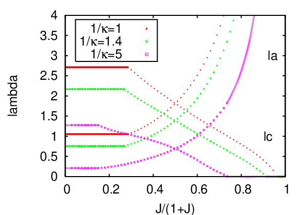
We have no physical explanation for the behaviour of $\lambda_{a}$ , $\lambda_{c}$ as functions of $J$ and $\kappa$ but it is gratifying to see that $\lambda_{a}=\lambda_{c}$ at $J=1$ independent of $\kappa$ in accordance with earlier work Sachdev 1992.

As indicated above, along with numerical study of Eq. 11, we performed extensive analytical calculations, both to corroborate the numerics and to obtain additional insight into the problem. Details of the analytical techniques are presented in Appendix B. Here we state that we were able to analytically determine ${\rm Sp(\mathcal{N})}$ phase boundaries between the SRO and LRO DC phase, between the DC and IC phase, and between the FM and IC phase, see Fig. 9. Moreover, our analytical calculations allowed us to explicitly confirm the existence of LRO inside the FM phase and immediately to the right of the FM-IC phase boundary. Likewise, the regions with SRO and LRO inside and immediately to the left of IC-DC phase boundary were determined analytically. This was achieved by evaluating in these regions the ${\rm Sp(\mathcal{N})}$ generalisation of the spin-spin correlation function $\langle{\mathbf{S}}_{i,u}\cdot{\mathbf{S}}_{j,v}\rangle$ of the model defined by expression (13). ( $u,v=a,b,c$ denote the sites of the triangular cells $i$ and $j$ of the model, see Fig. 8). On the right-hand side of the FM-IC boundary and inside the FM phase, we find for large distances between the cells, $|\mathbf{r}_{j}-\mathbf{r}_{i}|\gg 1$ ,

	$\langle{\mathbf{S}}_{i,u}\cdot{\mathbf{S}}_{j,v}\rangle\sim S_{u}\;S_{v}\;,$	(26a)
where

	$\displaystyle S_{w}\sim\sqrt{\frac{3}{2}}\frac{\|x_{3}({\mathbf{k}_{min}})\|^{2}}{N_{\bigtriangledown}\,(\lambda_{c}+\lambda_{a})}\;\left\{\begin{array}[]{ll}\frac{\lambda_{c}}{2}&\quad w=a,b\\[8.61108pt] -\lambda_{a}&\quad w=c\end{array}\right.$

and $u,v=a,b,c$ denote the sites of the triangular cells $i$ and $j$ of the model, see Fig. 8. Here, $|x_{3}({\mathbf{k}_{min}})|^{2}/N_{\bigtriangledown}$ is the condensate density at ${\mathbf{k}_{min}}=(-\pi,0)$ , $|x_{3}({\mathbf{k}_{min}})|^{2}/N_{\bigtriangledown}=\kappa$ , see Eq. (59). On the FM-IC transition line and inside the FM phase, where Eqs. (26) are valid, the parameters $\lambda_{a}$ and $\lambda_{c}$ are not independent but can be expressed in terms of a single parameter $\delta$ , see Eqs. (55), (63). The sign pattern on the right-hand side of Eq. (26) and the ordering wave vector $\mathbf{q}_{ord}=2{\mathbf{k}_{min}}=(-2\pi,0)$ are indeed the properties one expects to find for the long-distance behaviour of the spin-spin correlation function of a ferrimagnetically ordered state. Since $|x_{3}({\mathbf{k}_{min}})|^{2}/N_{\bigtriangledown}$ remains finite for arbitrarily small values of $\kappa$ , the mean-field ${\rm Sp(\mathcal{N})}$ approach predicts that this order persists in the extreme quantum limit of our model, $1/\kappa\gg 1$ . Together with Eqs. (26), the fact that the condensate density $|x_{3}({\mathbf{k}_{min}})|^{2}/N_{\bigtriangledown}$ remains constant inside the FM region, see Eq. (59), implies that the magnetisation of the FM phase remains constant up to the FM-IC phase boundary. The same behaviour of the magnetisation of a ferrimagnetic phase has previously been observed in an exact-diagonalisation study of a one-dimensional kagomé-like antiferromagnet Waldtmann et al. 2000. At the FM-IC phase boundary, the magnetisation becomes spatially modulated with an incommensurate wave vector ${\mathbf{q}_{ord}}=2{\mathbf{k}_{min}}$ .
On the left-hand side of the IC-DC boundary and inside the DC phase we find the following large distance behaviour of the spin-spin correlation function:


$\displaystyle\langle{\mathbf{S}}_{i,c}\cdot{\mathbf{S}}_{j,c}\rangle\,$	$\displaystyle\sim$	$\displaystyle\,\frac{3}{2}\cos\left[2\,{\mathbf{k}_{min}}\,(\mathbf{r}_{i}-\mathbf{r}_{j})\right]\left(\frac{2q_{1}^{2}}{1+q_{1}^{2}}\right)^{2}$	(27a)
		$\displaystyle\cdot\;\left[\frac{\|x_{3}({\mathbf{k}_{min}})\|^{2}+\|x_{3}(-{\mathbf{k}_{min}})\|^{2}}{N_{\bigtriangledown}\,q_{2}^{2}\lambda_{a}\omega^{(2)}_{3}({\mathbf{k}_{min}})}\right]^{2}\,,$	(27a)
$\displaystyle\langle{\mathbf{S}}_{i,u}\cdot{\mathbf{S}}_{j,v}\rangle\,$	$\displaystyle\sim$	$\displaystyle\,0\qquad\mbox{for}\quad u,v\,\neq\,c,c\,.$	(27b)

Here, $q_{1}$ and $\lambda_{a}$ denote the saddle-point values of these variables obtained from Eqs. (82), (83). $q_{2}$ is a function of $q_{1}$ , determined by Eq. (87) or by Eq. (95) depending on whether $1/\kappa<1/\kappa_{s}$ or $1/\kappa>1/\kappa_{s}$ ( $\kappa_{s}=0.181$ , see Fig. 22). $\omega^{(2)}_{3}({\mathbf{k}_{min}})$ is the value of the second-order expansion coefficient of the lowest spinon frequency $\omega_{3}({\mathbf{k}})$ , cf. Eqs. (71), (72c), at its minimum, and $2\,{\mathbf{k}_{min}}$ is the ordering wave vector immediately to the left on the IC-DC phase boundary and inside the DC phase; it is determined by Eq. (86). $|x_{3}({\mathbf{k}_{min}})|^{2}/N_{\bigtriangledown}=|x_{3}(-{\mathbf{k}_{min}})|^{2}/N_{\bigtriangledown}$ are the condensate densities at the wave vectors $\pm{\mathbf{k}_{min}}$ . As is shown in Appendix B, $\omega^{(2)}_{3}({\mathbf{k}_{min}})$ remains finite for $1/\kappa>1/\kappa_{s}$ and hence $|x_{3}(\pm{\mathbf{k}_{min}})|^{2}/N_{\bigtriangledown}$ vanishes. Thus, $\langle{\mathbf{S}}_{i,c}\cdot{\mathbf{S}}_{j,c}\rangle\sim 0$ , i.e., there is no LRO in this region. By contrast, for $1/\kappa<1/\kappa_{s}$ both, $|x_{3}(\pm{\mathbf{k}_{min}})|^{2}/N_{\bigtriangledown}$ and $\bar{\omega}^{(2)}_{3}({\mathbf{k}_{min}})$ vanish when the IC-DC phase boundary is approached from the left. However their ratio, which determines the spin-spin-correlation function, Eqs. (27), remains finite in this limit according to Eq. (93). Thus, for $1/\kappa<1/\kappa_{s}$ , Eqs. (27) show that while the chain spins ${\mathbf{S}}_{a}$ , ${\mathbf{S}}_{b}$ remain disordered, there is long-range IC order between the middle spins ${\mathbf{S}}_{c}$ along the IC-DC phase boundary and inside the DC phase for sufficiently large $\kappa$ . The middle spins occupy the sites of a triangular lattice. Remarkably, the correlations between these spins predicted by Eqs. (27) are compatible with the spin pattern

{\mathbf{S}}_{j,c}=S\left[\cos(2{\mathbf{k}_{min}}\mathbf{r}_{j})\hat{\mathbf{e}}_{x}+\sin(2{\mathbf{k}_{min}}\mathbf{r}_{j})\hat{\mathbf{e}}_{y}\right]

(28)

that would obtain if the middle spins ${\mathbf{S}}_{c}$ were classical spins coupled by a classical Heisenberg model with exchange constant $\tilde{J}$ along one lattice direction and couplings $\tilde{J^{\prime}}$ along the other two directions with a ratio $\tilde{J^{\prime}}/\tilde{J}$ such that incommensurate order with wave vector $2{\mathbf{k}_{min}}$ would be established. This persistence of long range order in the DC phase of the AKAF distinguishes our result from the result obtained by Chung et al., Ref. Chung et al. 2001b, in their large- $\mathcal{N}$ ${\rm Sp(\mathcal{N})}$ treatment of the anisotropic triangular antiferromagnet: there the DC phase consists of uncorrelated linear spin chains. Qualitative considerations of the finite- $\mathcal{N}$ corrections to the mean-field ${\rm Sp(\mathcal{N})}$ result led the authors of Ref. Chung et al. 2001b to the conclusion that instead of the DC phase there is spin-Peierls order in the large– $J$ region of their model. In the next section, we will present a different approach, a block-spin perturbation theory, to get further insight into the properties of the AKAF for the physical spin-1/2 case.

IV Block-spin perturbation approach

The basic idea of the block-spin perturbation theory is to calculate the states of small clusters of a given lattice exactly and to treat the coupling between these clusters perturbatively. The basic building blocks of the kagomé lattice are triangles. Thus it is natural to consider the trimerised kagomé lattice in which the spins on the downward pointing triangles are assumed to be strongly coupled whereas the coupling on the bonds of the upward pointing triangles are assumed to be weak, see Fig. 14. (Clearly, the exchange of the roles of the upward and the downward pointing triangles will not affect the further development to be presented in the current section.) The Hamiltonian for this trimerised model reads

\mathcal{H}(J,\gamma)=\mathcal{H}_{\bigtriangledown}(J)+\gamma\mathcal{H}_{\bigtriangleup}(J)\,,\,\,\,0\leq\gamma\leq 1\,,

(29)

where $\mathcal{H}_{\bigtriangledown}(J)$ ( $\mathcal{H}_{\bigtriangleup}(J)$ ) denote those terms in the Hamiltonian (Eq. 1) that act on the bonds of the downward (upward) pointing triangles. We will determine approximate GSs of this trimerised model in different ranges of $J$ in a perturbation expansion w.r.t. $\gamma$ . The hope is that the results will provide some qualitative insight into the GS properties of the non-trimerised model $\mathcal{H}(J,1)$ which is our original model Eq. (1). The same strategy has previously been applied sucessfully to frustrated spin models by several authors Subrahmanyam 1995; Mila 1998; Raghu et al. 2000; Zhitomirsky 2005.

Obviously, the GSs of the unperturbed Hamiltonian $\mathcal{H}(J,0)$ are products of GSs of the individual downward pointing triangular plaquettes. The GSs of a single plaquette and the corresponding energies are

for $J<1$ :

	${\left\|\alpha\right>}=\frac{1}{\sqrt{6}}\Big[\big({\left\|\uparrow\uparrow\downarrow\right>}-{\left\|\downarrow\uparrow\uparrow\right>}\big)+\big({\left\|\uparrow\downarrow\uparrow\right>}-{\left\|\downarrow\uparrow\uparrow\right>}\big)\Big]\,,$		(30a)
	${\left\|\bar{\alpha}\right>}=\frac{1}{\sqrt{6}}\Big[\big({\left\|\downarrow\downarrow\uparrow\right>}-{\left\|\uparrow\downarrow\downarrow\right>}\big)+\big({\left\|\downarrow\uparrow\downarrow\right>}-{\left\|\uparrow\downarrow\downarrow\right>}\big)\Big]\,,$		(30b)
	$\varepsilon_{\alpha}=\varepsilon_{\bar{\alpha}}=-1+J/4\,;$		(30c)

$J>1$ :

	${\left\|\beta\right>}=\frac{1}{\sqrt{2}}\big({\left\|\uparrow\downarrow\uparrow\right>}-{\left\|\uparrow\uparrow\downarrow\right>}\big)\,,$		(31a)
	${\left\|\bar{\beta}\right>}=\frac{1}{\sqrt{2}}\big({\left\|\downarrow\uparrow\downarrow\right>}-{\left\|\downarrow\downarrow\uparrow\right>}\big)\,,$		(31b)
	$\varepsilon_{\beta}=\varepsilon_{\bar{\beta}}=-3/4J\,.$		(31c)

Here, the ket vectors denote the spin state of the plaquette in the $S^{z}$ basis. The three arrows inside the ${\left|cba\right>}$ symbol denote from left to right the spin direction at the sites $c$ , $b$ and $a$ of the plaquettes in Fig. 15. The states ${\left|\alpha\right>}$ ( ${\left|\bar{\alpha}\right>}$ ) and ${\left|\beta\right>}$ ( ${\left|\bar{\beta}\right>}$ ) have total z-spin $1/2$ ( $-1/2$ ). They can be depicted graphically as shown in Fig. 15. From these plaquette states, the zeroth order GSs of the Hamiltonian $\mathcal{H}(J,\gamma)$ will be constructed. We treat the cases $J<1$ and $J>1$ separately.

$J<1$ :

Since the states ${\left|\alpha\right>}$ , ${\left|\bar{\alpha}\right>}$ are the GSs of the individual downward pointing plaquettes in this case, the states

{\left|A(M)\right>}=\prod_{i\epsilon\{M\}}{\left|\alpha_{i}\right>}\prod_{j\epsilon\{N_{\bigtriangledown}-M\}}{\left|\bar{\alpha}_{j}\right>}\,,

(32)

are here the zeroth order GSs of $\mathcal{H}(J,\gamma)$ . The set $\{M\}$ is a subset of $M$ out of the $N_{\bigtriangledown}$ downward pointing triangles of the $3N_{\bigtriangledown}$ -site kagomé lattice; the subscripts $i$ , $j$ denote the position of individual triangular plaquettes in the lattice of these plaquettes which is also triangular, see Fig. 14. The zeroth order energy eigenvalues associated with the states ${\left|A(M)\right>}$ do not depend on $M$ :

E^{(0)}_{A(M)}=N_{\bigtriangledown}(-1+J/4)\,.

(33)

Hence, there are in total $2^{N_{\bigtriangledown}}$ degenerate zeroth order GSs ${\left|A(M)\right>}$ . The single plaquette states ${\left|\alpha\right>}$ , ${\left|\bar{\alpha}\right>}$ satisfy the conditions for the validity of the Lieb-Mattis theorem, Ref. Lieb and Mattis 1962: after a canonical transformation which rotates the spins on the sites $a$ and $b$ by $\pi$ around the z-axis ${\left|\uparrow\right>}\rightarrow i{\left|\uparrow\right>}$ , ${\left|\downarrow\right>}\rightarrow-i{\left|\downarrow\right>}$ , and which leaves the spins on the site $c$ fixed the coefficients of all basis states on the right sides of Eqs. (30a, 30b) become positive ( $+1/\sqrt{6}$ ). As a consequence, all the GSs ${\left|A(M)\right>}$ satisfy the conditions for the validity of the Lieb-Mattis theorem. For $J=0$ it follows from this theorem that the total magnetisation of the exact quantum GS ${\left|\Phi_{exact}\right>}$ of the Hamiltonian $\mathcal{H}_{\rm AKAF}$ must be an eigenstate of the total magnetisation

\hat{m}_{tot}=\sum_{i}^{N_{\bigtriangledown}}(S^{z}_{i,a}+S^{z}_{i,b}+S^{z}_{i,c})

(34)

with eigenvalue $m_{tot}=N_{\bigtriangledown}/2$ , i.e., ${\left|\Phi_{exact}\right>}$ must be a ferrimagnetic state. By continuity, one expects this to be the case not only for $J=0$ , but up to a certain finite value of $J$ . This suggests that the state ${\left|A(M\!=\!0)\right>}$ , c.f. Eq (32), is the appropriate zeroth order GS in this case and that the degeneracy of the states ${\left|A(M)\right>}$ is lifted by the perturbation $\mathcal{H}_{\bigtriangleup}$ in favour of the state ${\left|A(0)\right>}$ . To confirm this, we determine the creation energy of a flipped plaquette in first order in $\gamma$ , i.e., the difference of the energy of the state with one plaquette spin flipped relative to the ferrimagnetic state, and the energy of the ferrimagnetic state:

\delta^{(1)}E_{A}({M\!=\!1)}=E_{A(1)}-E_{A(0)}.

(35)

A simple calculation yields

\delta^{(1)}E_{A}({M\!=\!1)}=\frac{4}{9}\gamma(1-J)\,,

(36)

i.e., to first order, ${\left|A(M\!=\!0)\right>}$ , the ferrimagnetic GS is stable w.r.t. a flip of a single plaquette spin, as long as $J<1$ .

As a further check on the stability of the state ${\left|A(M\!=\!0)\right>}$ , we calculate the dispersion of the excitation energy of a propagating single flipped plaquette spin. For this purpose, we need to determine the overlap matrix elements between the state with a flipped plaquette spin at the site $j$ and states with a flipped spin at one of the neighbouring sites,

	$t_{j,j\pm\mbox{\boldmath{\scriptsize$\delta$}}_{1}}={\left<\bar{\alpha}_{j}\right\|}{\left<\alpha_{j\pm\mbox{\boldmath{\scriptsize$\delta$}}_{1}}\right\|}\gamma J{\mathbf{S}}_{j}{\mathbf{S}}_{j\pm\mbox{\boldmath{\scriptsize$\delta$}}_{1}}{\left\|\alpha_{j}\right>}{\left\|\bar{\alpha}_{j\pm\mbox{\boldmath{\scriptsize$\delta$}}_{1}}\right>}=\frac{2}{9}\gamma J\,,\\$		(37a)
	$t_{j,j\pm\mbox{\boldmath{\scriptsize$\delta$}}_{2,3}}={\left<\bar{\alpha}_{j}\right\|}{\left<\alpha_{j\pm\mbox{\boldmath{\scriptsize$\delta$}}_{2,3}}\right\|}\gamma{\mathbf{S}}_{j}{\mathbf{S}}_{j\pm\mbox{\boldmath{\scriptsize$\delta$}}_{2,3}}{\left\|\alpha_{j}\right>}{\left\|\bar{\alpha}_{j\pm\delta_{2,3}}\right>}=-\frac{1}{9}\gamma\,.$		(37b)

Here, $\mbox{\boldmath{$\delta$}}_{\nu},\;\nu\,=\,1,\,2,\,3,$ are the primitive lattice vectors of the kagomé net, see Fig. 2; they connect the sites of the plaquette lattice. Then, by diagonalising the ensuing transfer Hamiltonian

$\displaystyle\mathcal{H}_{trans}=\gamma\sum_{j}\Big\{$	$\displaystyle\frac{2}{9}J\left(\,{\left\|j+\mbox{\boldmath{$\delta$}}_{1}\right>}{\left<j\right\|}+{\left\|j-\mbox{\boldmath{$\delta$}}_{1}\right>}{\left<j\right\|}\,\right)$	(38)
	$\displaystyle-\frac{1}{9}\left({\left\|j+\mbox{\boldmath{$\delta$}}_{2}\right>}{\left<j\right\|}+{\left\|j-\mbox{\boldmath{$\delta$}}_{2}\right>}{\left<j\right\|}\right)$
	$\displaystyle-\frac{1}{9}\left({\left\|j+\mbox{\boldmath{$\delta$}}_{3}\right>}{\left<j\right\|}+{\left\|j-\mbox{\boldmath{$\delta$}}_{3}\right>}{\left<j\right\|}\right)\,\Big\}\,,$

where ${\left|j\right>}$ denotes the state with a flipped plaquette spin at site $j$ , we obtain for the kinetic energy of this excitation:

\varepsilon({{\mathbf{k}}})=\frac{4}{9}\gamma\left[J\cos(k_{x})-\cos(\frac{k_{x}}{2})\cos(\frac{\sqrt{3}k_{y}}{2})\right]\,.

(39)

Adding the energy for the creation of a single flipped plaquette spin, we find for the total energy of the excitation in the limit of small wave vector ${\mathbf{k}}$

\omega({{\mathbf{k}}})=\frac{2}{9}\gamma\left[\,(\frac{1}{4}-J)k^{2}_{x}+\frac{3}{4}k^{2}_{y}+{\mathcal{O}}(k^{4})\,\right]\;.

(40)

Obviously, the ferrimagnetic state ${\left|A(M\!=\!0)\right>}$ becomes unstable against a propagating flipped plaquette spin already at $J=1/4$ , i.e., much earlier than suggested by the excitation energy of a static flipped spin (see Eq. (36)). We remark that this bound is independent of the actual magnitude of the perturbation parameter $\gamma$ and therefore, the qualitative result may survive in the limit $\gamma=1$ .

$J>1$ :

In this region, the states

{\left|B(M)\right>}=\prod_{i\epsilon\{M\}}{\left|\beta_{i}\right>}\prod_{j\epsilon\{N_{\bigtriangledown}-M\}}{\left|\bar{\beta}_{j}\right>}

(41)

with eigenenergy

E^{(0)}_{B(M)}=N_{\bigtriangledown}(-3J/4)\,.

(42)

are the zeroth order eigenstates of $\mathcal{H}(J,\gamma)$ . These states consist of free spins on the $c$ -sites and of spin-singlet dimers that cover every second bond of the horizontal chains of the lattice. We wish to answer the question of whether the $2^{N_{\bigtriangledown}}$ -fold degeneracy of these states, which results from the degrees of freedom of the free spins, is lifted by the perturbation $\gamma\mathcal{H}_{\bigtriangleup}$ ; in other words, we want to find out whether the middle spins remain decoupled from the chain spins. We proceed as in case (i). We compare in a perturbation expansion w.r.t. $\gamma$ the energy of the state ${\left|B(0)\right>}$ with the energy of ${\left|B(1)\right>}$ , i.e. with the state with one plaquette spin flipped relative to ${\left|B(0)\right>}$ . We denote this difference by $\delta^{(1)}E_{B}(M\!=\!1)=E_{B(1)}-E_{B(0)}$ . Surprisingly, we find that the matrix elements ${\left<B(M)\right|}\mathcal{H}_{\bigtriangleup}{\left|B(M)\right>}$ vanish for any choice of $M$ . There is no first order correction to the energy $E^{(0)}_{B(M)}$ , $\delta^{(1)}E_{B}(M\!=\!1)=0$ . Moreover, we observe that the off-diagonal matrix elements ${\left<B^{\prime}(M)\right|}\mathcal{H}_{\bigtriangleup}{\left|B(M)\right>}$ , where ${\left|B^{\prime}(M)\right>}$ and ${\left|B(M)\right>}$ contain identical numbers of states ${\left|\beta\right>}$ , ${\left|\bar{\beta}\right>}$ but differ in their distribution over the $N_{\bigtriangledown}$ downward pointing triangles, also vanish. This implies that, in contrast to case (i), a flipped plaquette spin cannot hop to a neighbouring site in a first order process. Coupling between the spins on the $c$ -sites occurs only in second order in $\gamma$ . It is succinctly described by an effective spin Hamiltonian for the $c$ -site spins, which are at the same time total spins of the downward pointing plaquettes (see Fig. 15):

	$\displaystyle\mathcal{H}_{eff}=\sum_{i\,\in\,c}\;\sum_{\nu\,=\,1}^{3}$		$\displaystyle\Big\{J_{\mbox{\boldmath{\scriptsize$\delta$}}_{\nu}}^{\\|}\;S_{i}^{z}\,S_{i+\mbox{\boldmath{\scriptsize$\delta$}}_{\nu}}^{z}$		(43)
		$\displaystyle+$	$\displaystyle J_{\mbox{\boldmath{\scriptsize$\delta$}}_{\nu}}^{\bot}\left(S_{i}^{x}\,S_{i+\mbox{\boldmath{\scriptsize$\delta$}}_{\nu}}^{x}\,+\,S_{i}^{y}\,S_{i+\mbox{\boldmath{\scriptsize$\delta$}}_{\nu}}^{y}\right)\Big\}\,.$		(43)

Here, $S_{i}^{\alpha}$ , $\alpha=x$ , $y$ , $z$ , denote plaquette spin operators; $i$ is the position of a downward pointing plaquette on the triangular lattice formed by these plaquettes. The exchange couplings $J_{\mbox{\boldmath{\scriptsize$\delta$}}_{\nu}}^{\|}$ and $J_{\mbox{\boldmath{\scriptsize$\delta$}}_{\nu}}^{\bot}$ are given as second order matrix elements of $\mathcal{H}_{\bigtriangleup}$ :


$\displaystyle J^{\\|}_{\mbox{\boldmath{\scriptsize$\delta$}}_{\nu}}$	$\displaystyle=$	$\displaystyle\gamma^{2}\left\{\sum_{X}\frac{{\left<B_{i\uparrow,\,i^{\prime}\uparrow}\right\|}\mathcal{H}_{\bigtriangleup}{\left\|X\right>}\,{\left<X\right\|}\mathcal{H}_{\bigtriangleup}{\left\|B_{i\uparrow,\,i^{\prime}\uparrow}\right>}}{2\,\varepsilon_{B}-\varepsilon_{X}}\right.$	(44a)
		$\displaystyle\left.-\sum_{Y}\frac{{\left<B_{i\uparrow,\,i^{\prime}\downarrow}\right\|}\mathcal{H}_{\bigtriangleup}{\left\|Y\right>}\,{\left<Y\right\|}\mathcal{H}_{\bigtriangleup}{\left\|B_{i\uparrow,\,i^{\prime}\downarrow}\right>}}{2\,\varepsilon_{B}-\varepsilon_{Y}}\right\}$	(44a)

$\displaystyle J^{\bot}_{\mbox{\boldmath{\scriptsize$\delta$}}_{\nu}}$	$\displaystyle=$	$\displaystyle\gamma^{2}\sum_{X}\frac{{\left<B_{i\downarrow,\,i^{\prime}\uparrow}\right\|}\mathcal{H}_{\bigtriangleup}{\left\|X\right>}\,{\left<X\right\|}\mathcal{H}_{\bigtriangleup}{\left\|B_{i\uparrow,\,i^{\prime}\downarrow}\right>}}{2\,\varepsilon_{B}-\varepsilon_{X}}\,,$	(44b)

and $i^{\prime}\!\equiv\!i\!+\!\mbox{\boldmath{$\delta$}}_{\nu}$ . Here, the states ${\left|B_{i\sigma,\,i^{\prime}\sigma^{\prime}}\right>}$ are zeroth order GSs, Eq. (41), whose spin patterns are identical on all sites except for the sites $i$ and $i^{\prime}$ where the $z$ -components of the spins take the values $\sigma$ and $\sigma^{\prime}$ , respectively; ${\left|X\right>}$ and ${\left|Y\right>}$ are excited states of $\mathcal{H}_{\bigtriangledown}$ . Of course, since the ${\rm SU(2)}$ symmetry of the original Hamiltonian $\mathcal{H}(J,\gamma)$ must be conserved in the derivation of $\mathcal{H}_{eff}$ , the expressions Eqs. (44) must yield identical results, $J_{\mbox{\boldmath{\scriptsize$\delta$}}_{\nu}}^{\|}\,=\,J_{\mbox{\boldmath{\scriptsize$\delta$}}_{\nu}}^{\bot}\equiv J_{\mbox{\boldmath{\scriptsize$\delta$}}_{\nu}}$ . Non-zero contributions to $J^{\|}_{\mbox{\boldmath{\scriptsize$\delta$}}_{\nu}}$ and $J^{\bot}_{\mbox{\boldmath{\scriptsize$\delta$}}_{\nu}}$ are obtained if either the same term ${\mathbf{S}}_{i}{\mathbf{S}}_{i^{\prime}}$ of $\mathcal{H}_{\bigtriangleup}$ acts in both matrix elements of the numerators of Eq. (44) (two-block contributions) or the terms ${\mathbf{S}}_{i}{\mathbf{S}}_{k}$ , ${\mathbf{S}}_{k}{\mathbf{S}}_{i^{\prime}}$ act in the left and right elements, respectively, where the plaquette geometry must be as shown in Fig. 16 (three-block contributions). In contrast to the case of the isotropic KAF studied by Zhitomirsky Zhitomirsky 2005, the three-block contributions do not produce three-spin interactions in the present case. Rather, they contribute to the exchange interactions $J_{\mbox{\boldmath{\scriptsize$\delta$}}_{1}}^{\|}$ and $J_{\mbox{\boldmath{\scriptsize$\delta$}}_{1}}^{\bot}$ of the Hamiltonian $\mathcal{H}_{eff}$ , Eq. (43). The evaluation of the expressions (44) yields

	$\displaystyle J_{\mbox{\boldmath{\scriptsize$\delta$}}_{1}}$	$\displaystyle=$	$\displaystyle\;\;\gamma^{2}\,\frac{1}{288}\,\frac{1}{J}\left[\frac{56}{1-\frac{1}{J}}-\frac{1}{1-\frac{1}{4J}}+\frac{98}{1+\frac{1}{2J}}\right]$		(45)
		$\displaystyle=$	$\displaystyle\quad\frac{17}{32}\frac{\gamma^{2}}{J}\,\left[1+\mathcal{O}(J^{-1})\right]$		(45)

and

	$\displaystyle J_{\mbox{\boldmath{\scriptsize$\delta$}}_{2}}\,=\,J_{\mbox{\boldmath{\scriptsize$\delta$}}_{3}}\,$	$\displaystyle=$	$\displaystyle\,\frac{\gamma^{2}}{6J}\left[\frac{1}{1-\frac{1}{J}}\,-\,\frac{1}{1+\frac{1}{2J}}\right]$		(46)
		$\displaystyle=$	$\displaystyle\,\frac{\gamma^{2}}{4J^{2}}\left[1\,+\,\mathcal{O}(J^{-1})\right]\,.$		(46)

Figure 17: (Color online) Collinear antiferromagnetic state (CAF) on the triangular lattice Starykh and Balents 2007.

Obviously, these results are useful for $J\,\gg 1$ . There, $\mathcal{H}_{eff}$ represents a spin $1/2$ Heisenberg Hamiltonian on the triangular lattice of the $c$ -sites with a coupling along the $\mbox{\boldmath{$\delta$}}_{1}$ direction that is strong ( $\mathcal{O}(\gamma^{2}/J)$ ) in comparison to the couplings in the two other directions ( $\mathcal{O}(\gamma^{2}/J^{2})$ ). This limiting case of the anisotropic triangular Heisenberg antiferromagnet (ATHAF) has recently been analysed by Starykh and Balents with field theoretical methods Starykh and Balents 2007. These authors find that in the limit of strong anisotropy, $K\equiv J_{\mbox{\boldmath{\scriptsize$\delta$}}_{1}}/J_{\mbox{\boldmath{\scriptsize$\delta$}}_{2}}\rightarrow\infty$ , the GS of the model Eq. (43) is a collinearly ordered antiferromagnet (CAF) as depicted in Fig. 17. Since the ordering wave vector ${\mathbf{q}}_{CAF}\,=\,(\pi,\pi/2)$ of this phase does not evolve continuously from the ordering wave vector ${\mathbf{q}}_{IC}$ of the incommensurate (IC) spiral phase of the ATHAF, ( ${\mathbf{q}}_{IC}\,=\,(q_{x}(K),0)$ with $-3\pi/2\leq q_{x}(K)\leq-\pi$ for $1/2\leq K\leq\infty$ ), they conclude that the IC phase and the CAF phase must be separated by a quantum phase transition. For the trimerised anisotropic kagomé model, Eq. 29, these results have the following implications:
i) While in the limit of strong anisotropy $J\gg 1$ there is long-range collinear antiferromagnetic order among the $c$ -site spins, the $a$ - and $b$ -site spins are paired in singlets, see Fig. 18.
ii) This picture of the GS of the trimerised anisotropic kagomé model Eq. (29) differs from the result obtained in the ${\rm Sp(\mathcal{N})}$ approach insofar as for sufficiently large $\kappa$ the ${\rm Sp(\mathcal{N})}$ approach predicts long range IC order among the $c$ -site spins up to arbitrarily large values of $J$ . Thus, if the picture of a CAF phase for large anisotropy persists in the non-trimerised limit $\mathcal{H}(J,\gamma=1)$ of the model Eq. 29, one would expect a quantum phase transition between the IC phase and the CAF phase of the AKAF similarly as for the ATHAF. In closing this section, we remark that the calculation that led to the effective Hamiltonian $\mathcal{H}_{eff}$ , Eq. 43, i.e., to the coupling between the $c$ spins in the strongly anisotropic limit, shows clearly that this coupling arises from quantum fluctuations of the $a$ and $b$ spins.

V Summary and discussion

In this work, we have studied the ground state (GS) phase diagram of the quantum Heisenberg antiferromagnet on the kagomé lattice with spatially anisotropic exchange (AKAF). The model is relevant for a description of magnetic properties of volborthite, which is a natural realisation of a spin $1/2$ antiferromagnet consisting of weakly coupled slightly distorted kagomé layers. A small monoclinic distortion along one of the three lattice directions causes the exchange coupling along this direction, $J$ , to differ from the couplings in the other two directions, $J^{\prime}$ , which we set equal to unity, cf. Fig. 2. We have investigated the problem in the full range of the anisotropy, $0\leq J\leq\infty$ , using three different approximate methods: the classical and semiclassical approach, the mean-field ${\rm Sp(\mathcal{N})}$ approach, and a block-spin perturbation theory.

The case $J=1$ is the much studied isotropic kagomé antiferromagnet (KAF). Exact diagonalisation studies of this model Lecheminant et al. 1997; Waldtmann et al. 1998 are available. Their results speak conclusively in favour of a spin liquid ground state Misguich and Lhuillier 2004. This view is supported by block-spin approaches Mila 1998; Mambrini and Mila 2000. Conflicting results have been found in Refs. Marston and Zeng 1991; Zeng and Elser 1995; Syromyatnikov and Maleyev 2002; Nikolic and Senthil 2003; Budnik and Auerbach 2004, where various valence bond crystal (VBC) states are proposed as ground states of the KAF. However, a recent comparison of the exact spectrum of the 36-site sample of the KAF against the excitation spectra allowed by the symmetries of these states, casts doubts on their validity Misguich and Sindzingre 2007.

Within the whole anisotropy range, the case $J=0$ is special, since it allows for an exact characterisation of the quantum GS as ferrimagnetic (FM) with a total magnetisation of $M=S\,N_{s}/3$ for a system of $N_{s}$ spins of magnitude $S$ . In the classical picture, this state corresponds to a unique staggered layout of spins with a non-zero net magnetisation of the lattice unit cell (cf. Fig. 3). In the classical limit, the ferrimagnetic ground state survives up to $J=1/2$ . For $J>1/2$ , the “chain” spins (i.e., spins coupled by $J$ ) begin to tilt gradually towards the middle (remaining) spins (see Fig. 5). This allows for a formation of a large degenerate manifold of canted spin states. In contrast to the isotropic case $J=1$ , where the degeneracy grows exponentially with the system size $N_{s}$ , its growth is weaker: $2^{1.26\sqrt{N_{s}}}$ for $J\not=1$ . This implies that there must be an increasingly large number of classical low energy configurations as $J$ approaches unity. In the linear semiclassical approximation, the spin-wave spectrum has one zero-frequency mode for each point of the magnetic Brillouin zone (BZ). The spectrum is identical for the different canted states for all $J>1/2$ . Thus, in this order of the semiclassical approximation, no order-by-disorder mechanism appears that would select one particular state or a particular group of states from the manifold of canted states as true ground states. In the limit $J\rightarrow\infty$ , the frequency spectrum of non-zero modes gradually takes the shape of the spectrum that one would expect for a set of uncoupled antiferromagnetic spin chains parallel to the strong- $J$ direction. No qualitative change from the set of canted spin states to the set of decoupled chains at a finite value of $J$ is found.

We have further explored the nature of the phases at various $J$ exploiting the mean field (MF) ${\rm Sp(\mathcal{N})}$ approach, that incorporates the effect of quantum fluctuations not only perturbatively, but self-consistently. The strength of quantum fluctuations is controlled by a parameter $\kappa$ , which is the analogue of the spin value $S$ in the original ${\rm SU(2)}$ symmetric model. In fact, for $\mathcal{N}=1$ , when the ${\rm Sp(1)}$ symmetric model is equivalent to the ${\rm SU(2)}$ model, $\kappa=2S$ . For general $\mathcal{N}$ , this last identity does not hold, but $\kappa$ is still a measure for the importance of quantum fluctuations that are strong for $\kappa\ll 1$ and weak for $\kappa\gg 1$ . In the MF ${\rm Sp(\mathcal{N})}$ approach, the nature of the phases that occur can be read from the values of the mean field parameters $Q_{1}$ and $Q_{2}$ and from the spectrum of the bosonic spinon excitations. While the mean field parameters $Q_{1}$ and $Q_{2}$ (cf. Fig. 8) are the GS expectation values of singlet bond operators, the structure of the spinon spectrum, $\omega_{\mu}({\mathbf{k}};Q,\lambda)$ , determines the existence or non existence of long-range order (LRO): If the spectrum becomes gapless at some wavevector ${\mathbf{q}_{ord}}$ , a Bose condensate will form and a modulated structure with the wavevector $2{\mathbf{q}_{ord}}$ will acquire LRO.

As was to be expected, the phase diagram of the AKAF obtained by the MF ${\rm Sp(\mathcal{N})}$ approach contains an incommensurate (IC) phase in the vicinity of the isotropic point $J=1$ which is ordered for sufficiently large $\kappa$ according to this approach, see Fig. 9. Qualitatively, we may gauge the value of $\kappa$ against the spin length $S$ by looking at the line $J=1$ of the phase diagram which is the location of the ${\rm Sp(\mathcal{N})}$ analogue of the isotropic ${\rm SU(2)}$ symmetric kagomé model: since, as we have argued above, the ${\rm SU(2)}$ model is disordered for $S=1/2$ , we may conclude from Fig. 9 that the value of $1/\kappa$ that corresponds to $S=1/2$ must be greater than two. Somewhat surprisingly, the FM phase remains long-range ordered for arbitrarily small $\kappa$ . This may reflect the fact that in the ${\rm SU(2)}$ version of the model, the FM phase is ordered even for the smallest physical spin value $S=1/2$ . A new feature of the phase diagram is the prediction of a decoupled chain (DC) phase for large enough $J$ , which has no classical analogue. In this phase, the chains of strongly coupled $a$ - and $b$ -site spins show no magnetic order. The $c$ -site spins which are interspersed between these chains and which occupy the sites of triangular sublattice are decoupled from the chain spins. However, they may or may not exhibit long range order among themselves depending on the magnitude of $\kappa$ . Remarkably, the spin-spin correlations, whose asymptotics were obtained analytically, are compatible with the spin-spin correlations of an anisotropic classical Heisenberg antiferromagnet on the triangular lattice whose exchange couplings differ in one direction from those in the other two directions.

In order to tackle the problem of the GSs of the AKAF from a third corner, we have used a block-spin perturbation theory. This method has the advantage of being applicable directly to the spin $1/2$ version of the model. In applying this approach, one has to initially group the spins of the model in clusters. For the kagomé lattice, it is natural to choose the spins around either the upward or the downward pointing triangles as clusters of strongly coupled units and to consider the coupling between these clusters, $\gamma$ , as the small expansion parameter. Thus one trimerises the original model (see Fig. 14) and in so doing, one breaks the translational invariance of the original model. In the zeroth order of this expansion, two regions can be distinguished by the eigenenergies of the individual trimers: $J<1$ and $J>1$ . For sufficiently small $J$ , one recovers the FM state as the GS in first order w.r.t. $\gamma$ . For $J>1$ , there are no first order corrections to the energy. Following an earlier application of the block-spin technique to the isotropic KAF Zhitomirsky 2005, we determine for $J>1$ in second order in $\gamma$ an effective Hamiltonian $\mathcal{H}_{eff}$ for the block-spins which can be identified as the middle spins of the original model and that occupy the sites of a triangular lattice. $\mathcal{H}_{eff}$ is a Heisenberg Hamiltonian with a coupling $J_{\mbox{\boldmath{\scriptsize$\delta$}}_{1}}$ of the order of $\gamma^{2}/J$ along the $\mbox{\boldmath{$\delta$}}_{1}$ direction (cf. Fig. 2) and couplings $J_{\mbox{\boldmath{\scriptsize$\delta$}}_{2}}=J_{\mbox{\boldmath{\scriptsize$\delta$}}_{3}}$ of the order of $\gamma^{2}/J^{2}$ along the other two directions. The calculations that lead to these results show clearly that the couplings between the $c$ -spins of the AKAF are due to fluctuations of the singlets between the $a$ - and $b$ -spins into excited states. In a very recent field theoretical study, Starykh and Balents Starykh and Balents 2007 arrive at the conclusion that for $J_{\mbox{\boldmath{\scriptsize$\delta$}}_{1}}\gg J_{\mbox{\boldmath{\scriptsize$\delta$}}_{2},\mbox{\boldmath{\scriptsize$\delta$}}_{3}}$ , the ground state of the anisotropic triangular antiferromagnet represented by $\mathcal{H}_{eff}$ is a collinearly ordered spin state, see Fig. 17. Then, together with the singlet dimers between the $a$ - and $b$ -spins of the downward pointing triangles, the state depicted in Fig. 18 emerges as the candidate ground state of the AKAF in the limit of large anisotropy $J\gg 1$ : while nearest neighbour spins on the strongly coupled $a$ - $b$ chains form singlets and decouple magnetically from the spins on the $c$ sites, the latter order in a collinear antiferromagnetic structure. This structure cannot be obtained by a continuous deformation of the spiral IC structure that is predicted by the ${\rm Sp(\mathcal{N})}$ approach and is believed to prevail for sufficiently large $\kappa$ in the region of moderate anisotropy. As a consequence of the trimerisation, the state depicted in Fig. 18 breaks the translational symmetry of our original model, Eq. (1). If this state survives as the ground state of the non-trimerised model, i.e., when the expansion parameter $\gamma$ approaches unity, then, owing to their incompatible symmetries, the spiral IC phase and the large J phase of our model must be separated by a quantum phase transition.

Acknowledgements.

One of the authors (HUE) acknowledges a useful discussion with F. Mila. The work at the University of Waterloo was supported by the Canada Research Chair (Tier I, Michel Gingras). We thank M. Gingras for a critical reading of the manuscript and numerous helpful suggestions.

Appendix A Ground state degeneracy for general $J$

We first derive the constraint on the chiralities that leads to the reduction in the number of degenerate ground states for general $J$ relative to the special case $J=1$ . Let $\chi_{1},\,\cdots,\,\chi_{6}$ be the chiralities of the six triangles surrounding one of the hexagons of the kagomé lattice, and let $\phi_{1},\,\cdots,\,\phi_{6}$ denote the angles that define the directions of the spin vectors on the six corners of the hexagon, see Fig. 19.

Then, as is seen in Fig. 19, the following relations between the angle $\phi_{1},$ and the angles $\phi_{2}\,\cdots,\,\phi_{6}$ are an immediate consequence of these definitions:


$\displaystyle\phi_{2}$	$\displaystyle=$	$\displaystyle\phi_{1}-\theta\,\chi_{2}\,,$	(47a)
$\displaystyle\phi_{3}$	$\displaystyle=$	$\displaystyle\phi_{1}-\theta\,(\chi_{2}+\chi_{3})\,,$	(47b)
$\displaystyle\phi_{4}$	$\displaystyle=$	$\displaystyle\phi_{1}-\theta\,(\chi_{2}+\chi_{3})-(2\pi\!-\!2\theta)\;\chi_{4}\,,$	(47c)
$\displaystyle\phi_{5}$	$\displaystyle=$	$\displaystyle\phi_{1}-\theta\,(\chi_{2}+\chi_{3}+\chi_{5})-(2\pi\!-\!2\theta)\;\chi_{4}\,,$	(47d)
$\displaystyle\phi_{6}$	$\displaystyle=$	$\displaystyle\phi_{1}-\theta\,(\chi_{2}+\chi_{3}+\chi_{5}+\chi_{6})-(2\pi\!-\!2\theta)\;\chi_{4},\qquad$	(47f)
		$\displaystyle\mbox{and}\quad\phi_{6}=\phi_{1}+(2\pi-2\theta)\chi_{1}\,.$	(47f)

From the last two of these relations it follows that the chiralities $\chi_{1},\,\cdots\,,\chi_{6}$ are constrained by the sum rule

\chi_{2}+\chi_{3}+\chi_{5}+\chi_{6}-2\,\chi_{1}-2\,\chi_{4}=0\,.

(48)

For the isotropic kagomé system, $J=1$ , $\theta=2\pi/3$ , one finds instead of the constraint (48) the sum rule

\sum_{j=1}^{6}\chi_{j}=n\quad\mbox{where}\quad n=0,\,1,\,2

(49)

which is obviously less restrictive than (48).
Next, we present the arguments that lead to the estimate

N^{aniso}_{GS}(N_{\bigtriangledown})\lesssim 2^{\alpha\sqrt{N_{\bigtriangledown}}}\quad\mbox{with}\quad\alpha<3

(50)

for the number $N^{aniso}_{GS}(N_{\bigtriangledown})$ of classical GSs of an anisotropic kagomé AF with $N_{\bigtriangledown}$ downward pointing triangles (the number of sites is $3N_{\bigtriangledown}$ ). Any planar configuration of a cell of the kagomé lattice can be constructed by decorating the successive rows of up and down pointing triangles with chirality values $\chi=\pm 1$ starting with the first row. We consider only square cells with $\sqrt{N_{\bigtriangledown}}$ rows with $\sqrt{N_{\bigtriangledown}}$ downward pointing triangles. Then, each row consists of $2\sqrt{N_{\bigtriangledown}}$ triangles, see Fig. 20.

Obviously, there are $2^{2\sqrt{N_{\bigtriangledown}}}$ ways to decorate the first row. Disregarding certain exceptions, which will be discussed below, one can, for a given configuration of the first row, choose the chirality of an arbitrary triangle of the second row to be either $+1$ or $-1$ . After this choice has been made, the constraint (48) fixes the chiralities of all the remaining triangles of the second row uniquely. Proceeding in this manner from row to row one would generate $2^{2\sqrt{N_{\bigtriangledown}}}\,\cdot\,2^{\sqrt{N_{\bigtriangledown}}}$ distributions of chiralities over the $N_{\bigtriangledown}$ downward pointing triangles of the cell. For finite lattice cells, the requirement of periodic boundary conditions imposes further constraints on the number of possible chirality distributions in these cells, but the effect of these constraints will become negligible in the thermodynamic limit $N_{\bigtriangledown}\rightarrow\infty$ . However, there is a further reduction of the number of possible chirality distributions: For a given distribution in a row it is not always possible to find two distributions for the successive row which both satisfy the constraint (48). If in a row the lower half of a hexagon of the next row is decorated by chiralities in the manner $-\,+\,-$ or $+\,-\,+$ (see boxes in Fig. 20), then the chiralities of the next row are fixed uniquely. This reduces the number of possible chirality distributions. Obviously, this reduction of the number of possible chirality distributions survives in the thermodynamic limit so that the exponent in (50) is less than $3\,\sqrt{N_{\bigtriangledown}}$ , the value one would have expected without this reduction. We have calculated the number of distributions for cells of up to $N_{\bigtriangledown}=13\times 13$ and have found the value $\alpha\simeq 2.18$ for the constant in the expression (50), see Fig. 21.

As we have mentioned above, the sum rule (49) which applies for the isotropic kagomé AF is less restrictive than the sum rule (48). Consequently, the number of chirality distributions in the isotropic model Baxter 1970,

N_{GS}^{iso}\sim 1.1833^{3N_{\bigtriangledown}}

(51)

is larger than in the anisotropic model. Since the transition from the anisotropic model to the isotropic model happens through a continuous variation of the coupling constant $J$ , there should be a continuous transition between the numbers of GS configurations in these two cases. Presumably, this transition implies that the density of low-energy states of the anisotropic model increases exponentially with an exponent $\sim\sqrt{N_{\bigtriangledown}}$ so that for $J\rightarrow 1$ a sufficient number of states collapses to the GS to bring about the transition between the laws (50) and (51).

Appendix B Phase boundaries

The FM phase and the DC phase are chacterised by the vanishing of the parameters $Q_{1}$ and $Q_{2}$ , respectively. Our numerical results in section III.3 show that at the respective phase boundaries, $Q_{1}$ and $Q_{2}$ decrease to zero like order parameters at second order phase transitions. This suggests that we expand the mean field energy $E_{\rm MF}$ , Eq. (14), w.r.t. either $Q_{1}$ or $Q_{2}$ in the manner of a Landau-Ginzburg (LG) expansion and determine the phase boundaries and the properties of the FM and the DC phase from this expansion. We write $E_{MF}/(N_{\bigtriangledown}\mathcal{N})=e^{(\alpha)}_{LG}(Q_{\alpha})$ where

e^{(\alpha)}_{LG}(Q_{\alpha})=e_{\alpha}+r_{\alpha}\,|Q_{\alpha}|^{2}+g_{\alpha}\,|Q_{\alpha}|^{4}+\mathcal{O}(|(Q_{\alpha}|^{6})\,.

(52)

The coefficients $e_{\alpha}$ , $r_{\alpha}$ and $g_{\alpha}$ are functions of the variables $\kappa$ and $J$ , of the parameters $\lambda_{a}$ , $\lambda_{c}$ and of $Q_{2}$ , $Q_{1}$ for $\alpha=1,\,2$ , respectively. The saddle point of $e^{(\alpha)}_{LG}(Q_{\alpha})$ w. r. t. $\lambda_{a}$ , $\lambda_{c}$ and $Q_{\beta}$ , $\beta\not=\alpha$ , determines the physical values of these parameters. For $e^{(\alpha)}_{LG}(Q_{\alpha})$ to qualify as a bona fide Landau-Ginzburg energy describing a second order phase transition with $Q_{\alpha}$ playing the role of an order parameter, the coefficients $g_{\alpha}$ have to be positive at the saddle point. For $g_{1}$ , i.e., inside and on the boundary of the FM phase, this follows from the numerical result: $Q_{1}$ is found to remain zero for all $J\leq J_{F}(\kappa)$ . By contrast, we have no numerical results for $J\geq J_{DC}(\kappa)$ , i.e., inside and on the boundary of the DC phase. Therefore, we need to show by analytic means that $g_{2}>0$ .

B.1 The FM phase and the FM-IC phase boundary

Since, as we have just remarked, we know that $g_{1}>0$ , the remaining task is to determine the coefficients $e_{1}$ and $r_{1}$ of $e^{(1)}_{LG}$ . To this end, we have to expand the mean field energy $E_{\rm MF}$ , Eq. (14), w.r.t. $Q_{1}$ which amounts to expanding the frequencies $\omega_{\mu}({\mathbf{k}})$ w.r.t. $Q_{1}$ . As can be inferred from the expressions (16), (III.2.1) the frequencies depend on $Q_{1}$ only through the combination $\varepsilon^{2}=J^{2}|\tilde{Q}_{1}|^{2}$ . Therefore, we write the expansion in the form

	$\displaystyle\omega_{\mu}({\mathbf{k}};\varepsilon)\,\,$	$\displaystyle=$	$\displaystyle\,\,\omega_{\mu}^{(0)}({\mathbf{k}})+\varepsilon^{2}\omega_{\mu}^{(1)}({\mathbf{k}})+\mathcal{O}(\varepsilon^{4})$		(53)
		$\displaystyle=$	$\displaystyle\,\,\lambda_{+}\left[\bar{\omega}_{\mu}^{(0)}({\mathbf{k}})+\bar{\varepsilon}^{2}\bar{\omega}_{\mu}^{(1)}({\mathbf{k}})+\mathcal{O}(\bar{\varepsilon}^{4})\right]$		(53)

with $\lambda_{+}=(\lambda_{a}+\lambda_{c})/2\,,\quad\bar{\omega}_{\mu}^{(0)}=\omega_{\mu}^{(0)}/\lambda_{+}\,,\quad\bar{\omega}_{\mu}^{(1)}({\mathbf{k}})=\lambda_{+}\,\partial_{\varepsilon^{2}}\,\omega_{\mu}({\mathbf{k}};\varepsilon)|_{\varepsilon=0}$ and $\bar{\varepsilon}=\varepsilon/\lambda_{+}$ .

Here, the introduction of the “dimensionless” quantities $\bar{\omega}_{\mu}^{(i)}$ , $\bar{\varepsilon}$ looks like an unneccessary complication but it will help to keep expressions further below simple. Setting $Q_{1}=0$ in the matrix $\hat{\mathbf{D}}(\omega)$ , Eq. (16), and solving Eq. (15) for $\omega$ we find


$\displaystyle\bar{\omega}_{1}^{(0)}({\mathbf{k}})\,\,$	$\displaystyle=$	$\displaystyle\,\,w_{F}({\mathbf{k}})+\delta\,,$	(54a)
$\displaystyle\bar{\omega}_{2}^{(0)}({\mathbf{k}})\,\,$	$\displaystyle=$	$\displaystyle\,\,1-\delta\,,$	(54b)
$\displaystyle\bar{\omega}_{3}^{(0)}({\mathbf{k}})\,\,$	$\displaystyle=$	$\displaystyle\,\,w_{F}({\mathbf{k}})-\delta\,.$	(54c)

Here

\delta\,=\,\lambda_{-}/\lambda_{+}\quad\mbox{with}\quad\lambda_{-}=(\lambda_{c}-\lambda_{a})/2

(55)

and

w_{F}({\mathbf{k}})\,=\,\sqrt{1-\bar{q_{2}}^{2}[\sin^{2}(s_{2}/2)+\sin^{2}(s_{3}/2)]}

(56)

with

	$\displaystyle\bar{q}_{2}=\|Q_{2}\|/\lambda_{+}\,$		(57)
	$\displaystyle\mbox{and}\quad\,\,s_{a}\,=\,{\mbox{\boldmath{$\delta$}}}_{a}\mathbf{k}\,,\,\,a=2,\,3\quad(\mbox{see Fig.~\ref{QP}})\,.$

From our numerical results, Fig. 13, we know that $\lambda_{c}>\lambda_{a}$ and hence $\delta>0$ . Therefore, $\bar{\omega}_{3}^{(0)}({\mathbf{k}})<\bar{\omega}_{1,2}^{(0)}({\mathbf{k}})$ , and hence, if the minimum of $\bar{\omega}_{3}^{(0)}({\mathbf{k}})$ vanishes at the point ${\mathbf{k}_{min}}$ in the Brillouin zone, $\bar{\omega}_{1,2}^{(0)}({\mathbf{k}_{min}})$ will be finite. Thus, since condensate can only occur when one of the frequencies $\bar{\omega}_{\mu}^{(0)}\,,\;\mu=1,\,2,\,3$ vanishes there may be a finite condensate density $|x_{3}({\mathbf{k}_{min}})|^{2}$ , but the densities $|x_{1}|^{2}$ and $|x_{2}|^{2}$ will certainly be zero. With these remarks and with the above results for $\bar{\omega}_{\mu}^{(0)}$ we find from Eq. (14)

$\displaystyle e_{1}/\lambda_{+}\;$	$\displaystyle=$	$\displaystyle\;2\lambda_{+}\bar{q}_{2}^{2}-(3-\delta)(\kappa+1)$	(58)
		$\displaystyle\;+\frac{1}{N_{\bigtriangledown}}\sum_{{\mathbf{k}}}\left[\bar{\omega}_{1}^{(0)}({\mathbf{k}})+\bar{\omega}_{2}^{(0)}({\mathbf{k}})+\bar{\omega}_{3}^{(0)}({\mathbf{k}})\right]$
		$\displaystyle\;+\bar{\omega}_{3}^{(0)}({\mathbf{k}_{min}})\,\|x_{3}({\mathbf{k}_{min}})\|^{2}/N_{\bigtriangledown}\,.$

Stationarity of $e_{1}$ w.r.t. $\lambda_{-}$ , $\lambda_{+}$ , and $\bar{q}_{2}^{2}$ (which is equivalent to stationarity w.r.t. $\lambda_{a}$ , $\lambda_{c}$ ), and $Q_{2}^{2}$ requires the following three conditions to be fulfilled:

	$\displaystyle\partial e_{1}/\partial\lambda_{-}=0:$
	$\displaystyle\mbox{\hskip 19.91692pt}\frac{1}{N_{\bigtriangledown}}\|x_{3}({\mathbf{k}}_{min})\|^{2}=\kappa\,;$		(59)
	$\displaystyle\partial e_{1}/\partial\lambda_{+}=0:$
	$\displaystyle\mbox{\hskip 19.91692pt}2\,\lambda_{+}\bar{q_{2}}^{2}-\frac{3}{2}\kappa-1+{\mathbf{E}}_{2}(\bar{q_{2}})+\frac{\kappa}{2}w_{F}({\mathbf{k}_{min}})=0\,;$
			(60)
	$\displaystyle\partial e_{1}/\partial\bar{q}_{2}^{2}=0:$
	$\displaystyle\mbox{\hskip 19.91692pt}2\,\lambda_{+}-\frac{1}{\bar{q_{2}}^{2}}\left[{\mathbf{K}}_{2}(\bar{q_{2}})-{\mathbf{E}}_{2}(\bar{q_{2}})\right]-\frac{\kappa}{w_{F}({\mathbf{k}_{min}})}=0\,;$
			(61)
	$\displaystyle\mbox{\hskip 19.91692pt}\mbox{with}\quad{\mathbf{K}}_{2}(\bar{q_{2}})=\frac{1}{\pi}\int_{0}^{\pi}\!\!ds_{2}\,\,\frac{1}{\pi}\int_{0}^{\pi}\!\!ds_{3}\;w_{F}({\mathbf{k}})^{-1}\,,$
	$\displaystyle\mbox{\hskip 19.91692pt}\mbox{\hskip 28.45274pt}{\mathbf{E}}_{2}(\bar{q_{2}})=\frac{1}{\pi}\int_{0}^{\pi}\!\!ds_{2}\,\,\frac{1}{\pi}\int_{0}^{\pi}\!\!ds_{3}\;w_{F}({\mathbf{k}})\,.$

According to Eq. (59), condensate must be present in the FM region. This requires that $\bar{\omega}_{3}^{(0)}({\mathbf{k}_{min}})$ vanishes. From Eq. (54c) it is seen that ${\mathbf{k}_{min}}=(-\pi,\,0)$ , so that $\bar{\omega}_{3}^{(0)}({\mathbf{k}_{min}})=0$ , if

w_{F}({\mathbf{k}_{min}})\;=\;\sqrt{1-2\bar{q_{2}}^{2}}\;=\;\frac{\lambda_{-}}{\lambda_{+}}\,.

(63)

Within the FM region and on the FM-IC boundary (i.e., for $Q_{1}=0$ ) the saddle-point values of $\bar{q_{2}}$ , $\lambda_{+}$ , and $\lambda_{-}$ are then determined as functions of $\kappa$ by the Eqs. (60), (61) and (63). Remarkably, within this region these quantities are independent of the value of the exchange constant $J$ . The solution of these equations shows that $0\leq\bar{q_{2}}\leq 2/3$ for $0<\kappa<\infty$ , cf. Figs. 11, 13.

The FM-IC phase boundary is the solution of $r_{1}(\kappa,J)=0$ (cf. Eq. (52), where

\left.r_{1}=\partial e^{(1)}_{LG}/\partial Q_{1}^{2}\right|_{Q_{1}=0}

(64)

with $e^{(1)}_{LG}$ ( $E_{\rm MF}$ ) from Eq. (14).

We obtain

	$\displaystyle\frac{r_{1}}{J^{2}}\;$	$\displaystyle=$	$\displaystyle\;\frac{1}{J}-\frac{1}{\lambda_{+}}\,\frac{1}{N_{\bigtriangledown}}\,\sum_{{\mathbf{k}}}\sin^{2}\left(\frac{s_{2}+s_{3}}{2}\right)\Omega^{(1)}({\mathbf{k}})$		(65)
			$\displaystyle+\frac{\kappa}{\lambda_{+}}\lim_{{\mathbf{k}}\rightarrow{\mathbf{k}}_{min}}\left(\sin^{2}\left(\frac{s_{2}+s_{3}}{2}\right)\bar{\omega}_{3}^{(1)}({\mathbf{k}})\right)$		(65)

with $\Omega^{(1)}({\mathbf{k}})=-\bar{\omega}_{1}^{(1)}({\mathbf{k}})-\bar{\omega}_{2}^{(1)}({\mathbf{k}})-\bar{\omega}_{3}^{(1)}({\mathbf{k}})$ .

To obtain the expansion coefficients $\bar{\omega}_{\mu}^{(1)}({\mathbf{k}})$ which appear in the last equation, we solve Eq. (15) to first order in the expansion w.r.t. $\bar{\varepsilon}^{2}$ . We find

	$\displaystyle\Omega^{(1)}({\mathbf{k}})$	$\displaystyle=$	$\displaystyle\left.\frac{1}{w_{F}({\mathbf{k}})(w_{F}({\mathbf{k}})+1-2\delta)}\right[w_{F}({\mathbf{k}})+1$
			$\displaystyle\left.+\frac{\bar{q_{2}}^{4}\,\sin^{2}\left(\frac{s_{2}}{2}\right)\,\sin^{2}\left(\frac{s_{3}}{2}\right)\,(2w_{F}({\mathbf{k}})+1-\delta)}{(w_{F}({\mathbf{k}})+1)(1-\delta)\,(w_{F}({\mathbf{k}})^{2}-\delta^{2})}\right]$

and

\lim_{{\mathbf{k}}\rightarrow{\mathbf{k}_{min}}}\left(\sin^{2}\left(\frac{s_{2}+s_{3}}{2}\right)\,\bar{\omega}_{3}^{(1)}({\mathbf{k}})\right)=-\frac{1}{2\delta}\,\frac{1+\delta}{1-\delta}\,.

(67)

With these results Eq. (65) can, in the thermodynamic limit, be cast into the form

\frac{r_{1}}{J^{2}}=\frac{1}{J}\,-\,\frac{I_{3}(\bar{q_{2}})}{\lambda_{+}}-\frac{\kappa}{\lambda_{+}}\,\frac{1}{2\delta}\,\frac{1+\delta}{1-\delta}=\frac{1}{J}-\frac{1}{J_{F}(\kappa)}\,,

(68)

where

I_{3}(\bar{q_{2}})=\frac{1}{\pi}\!\int_{0}^{\pi}\!\!\!ds_{2}\,\frac{1}{\pi}\!\int_{0}^{\pi}\!\!\!ds_{3}\,2\sin^{2}\left(\frac{s_{2}}{2}\right)\cos^{2}\left(\frac{s_{3}}{2}\right)\Omega^{(1)}({\mathbf{k}})\,.

(69)

Then, with $\bar{q}_{2}=\bar{q}_{2}(\kappa)$ and $\lambda_{\pm}=\lambda_{\pm}(\kappa)$ as obtained from Eqs. (60), (61) and (63), the condition $r_{1}\,=\,0$ is an equation for the FM-IC phase boundary $J=J_{F}(\kappa)$ which yields the graph shown in Fig. 9. As we have mentioned above, inside the FM region, i.e., for $J<J_{F}(\kappa)$ , the saddle-point values of the quantities $\bar{q}$ and $\lambda_{\pm}$ and hence of $Q_{2}$ , $\lambda_{a}$ , $\lambda_{c}$ and $|x_{3}({\mathbf{k}_{min}})|$ are independent of the exchange coupling $J$ , i.e., they retain the values they attain on the FM-IC phase boundary, cf. Figs. 11, 13.

B.2 The DC phase and the IC-DC phase boundary

Proceeding in exact analogy to the development in the previous subsection we now expand $E_{\rm MF}/(N_{\bigtriangledown}\,\mathcal{N})$ in powers of $|Q_{2}|^{2}$ . However, instead of working with the variables $Q_{1}$ , $Q_{2}$ , $\lambda_{a}$ , $\lambda_{c}$ we work with $q_{1}$ , $Q_{2}$ , $\lambda_{a}$ , $q_{2}$ here, where


$\displaystyle q_{1}$	$\displaystyle=$	$\displaystyle\frac{J\|Q_{1}\|}{\lambda_{a}}\,,$	(70a)
$\displaystyle q_{2}$	$\displaystyle=$	$\displaystyle\frac{\|Q_{2}\|}{\sqrt{\lambda_{a}\lambda_{c}}}\,.$	(70b)

The replacement of $|Q_{1}|$ is purely a matter of convenience. By contrast, the replacement of variables $Q_{2}$ , $\lambda_{c}$ , which according to the numerics vanish simultaneously as $J$ approaches the IC-DC phase boundary, by the pair $Q_{2}$ , $q_{2}$ leaves us with only one vanishing variable, since, as will be seen below, $q_{2}$ remains finite throughout.

B.2.1 Expansion of $e^{(2)}_{LG}(Q_{2})$

We write

\omega_{\mu}({\mathbf{k}})\,=\,\omega^{(0)}_{\mu}({\mathbf{k}})\,+\,\omega^{(2)}_{\mu}({\mathbf{k}})\,Q_{2}^{2}\,+\,\omega^{(4)}_{\mu}({\mathbf{k}})\,Q_{2}^{4}\,+\mathcal{O}(Q_{2}^{6})

(71)

and determine the coefficients $\omega^{(n)}_{\mu}$ , $n\,=\,1,\,\dots\,4,$ by solving Eq. (15) for $\omega$ iteratively. We obtain


	$\displaystyle\omega^{(0)}_{1}({\mathbf{k}})+\omega^{(0)}_{2}({\mathbf{k}})\,=2\lambda_{a}\,w_{DC}({\mathbf{k}})\,,\quad\omega^{(0)}_{3}=0\,,$		(72a)
	$\displaystyle\omega^{(2)}_{1}({\mathbf{k}})+\omega^{(2)}_{2}({\mathbf{k}})\,=\,-\frac{1}{\lambda_{a}}\,\frac{1-\cos k^{x}\,\cos k^{y}}{w_{DC}({\mathbf{k}})}\,,$		(72b)
	$\displaystyle\omega^{(2)}_{3}({\mathbf{k}})\,=\frac{1}{q_{2}^{2}\,\lambda_{a}}\,\left[C({\mathbf{k}})^{2}-D({\mathbf{k}})^{2}\right]^{1/2}\!\!.$		(72c)

Here,

C({\mathbf{k}})\;=\;1\,-\,q_{2}^{2}\;\frac{1\,-\,\cos k^{x}\,\cos k^{y}}{w_{DC}({\mathbf{k}})^{2}}\;,

(73)

D({\mathbf{k}})\;=\;q_{1}\sin k^{x}\;q_{2}^{2}\;\frac{\cos k^{x}-\cos k^{y}}{w_{DC}({\mathbf{k}})^{2}}\;,

(74)

w_{DC}({\mathbf{k}})\;=\;\sqrt{1-q_{1}^{2}\sin^{2}k^{x}}\,.

(75)

The coefficients $\omega^{(4)}_{\mu}({\mathbf{k}})$ , $\mu=1,\,2\,,3$ , will only be needed in the determination of the coefficient $g_{2}$ of the fourth order term of $e^{(2)}_{LG}(Q_{2})$ which will be discussed later. We will first concentrate on the determination of the zeroth order term, $e_{2}$ , and of the coefficient $r_{2}$ of the second order term of $e^{(2)}_{LG}(Q_{2})$ . Under the assumption that $g_{2}$ is positive, this will provide us with an expression for the IC-DC phase boundary.

With the above expressions for $\omega^{(\nu)}_{1}+\omega^{(\nu)}_{2}$ and $\omega^{(\nu)}_{3}$ , $\nu=0,\,1$ , we obtain for the coefficients of the Landau Ginzburg energy from Eqs. (14), (52)

e_{2}(q_{1},\lambda_{a})\;=\;\frac{\lambda_{a}^{2}\,q_{1}^{2}}{J}-2\lambda_{a}\left[1+\kappa-\frac{1}{N_{\bigtriangledown}}\sum_{{\mathbf{k}}}w_{DC}({\mathbf{k}})\right]\,,

(76)

	$\displaystyle\hskip-5.69054ptr_{2}(q_{1},\,q_{2},\,\lambda_{a},\,\|x_{3}({\mathbf{k}_{min}})\|^{2})\,=$
	$\displaystyle 2-\,\frac{1}{\lambda_{a}}\,\frac{1}{q_{2}^{2}}\,(\kappa\,+\,1)$
	$\displaystyle-\,\frac{1}{\lambda_{a}}\,\frac{1}{N_{\bigtriangledown}}\sum_{{\mathbf{k}}}\,\frac{1-\cos k^{x}\,\cos k^{y}}{w_{DC}({\mathbf{k}})}$
	$\displaystyle+\,\frac{1}{N_{\bigtriangledown}}\left[\sum_{{\mathbf{k}}}\,\omega^{(2)}_{3}({\mathbf{k}})+\|x_{3}({\mathbf{k}_{min}})\|^{2}\,\omega^{(2)}_{3}({\mathbf{k}_{min}})\right]\,.$		(77)

These are valid for arbitrary values of the parameters $q_{1}$ , $\lambda_{a}$ , $q_{2}$ , and $|x_{3}({\mathbf{k}_{min}})|$ . In the next subsection, we will calculate their saddle point values for given $Q_{2}$ and thus fix the parameters. Here, we have only allowed for the existence of a condensate component $|x_{3}({\mathbf{k}_{min}})|^{2}$ . This is justified since, as Eqs. (71) and (53) show, $\omega_{3}<\omega_{1,2}$ for sufficiently small $Q_{2}$ so that conceivably $\omega_{3}({\mathbf{k}})$ may vanish at some point ${\mathbf{k}_{min}}$ in the the Brillouin zone, while $\omega_{1}({\mathbf{k}})$ and $\omega_{2}({\mathbf{k}})$ remain finite at ${\mathbf{k}_{min}}$ , and hence a finite condensate density $|x_{3}({\mathbf{k}_{min}})|^{2}$ may occur at this point.

B.2.2 Saddle point, phase boundary

Next we need to determine the saddle point of $e^{(2)}_{LG}(Q_{2})$ in the space of the variables $q_{1}$ , $\lambda_{a}$ , $q_{2}$ , and $|x_{3}({\mathbf{k}_{min}})|$ . First, the saddle point values of $q_{1}$ and $\lambda_{a}$ are obtained as expansions in powers of $Q_{2}$ ,


$\displaystyle\lambda_{a}$	$\displaystyle=$	$\displaystyle\lambda_{a}^{(0)}+\lambda_{a}^{(2)}\,Q_{2}^{2}\,+\mathcal{O}(Q_{2}^{4})\,,$	(78a)
$\displaystyle q_{1}$	$\displaystyle=$	$\displaystyle q_{1}^{(0)}+q_{1}^{(2)}\,Q_{2}^{2}\,+\mathcal{O}(Q_{2}^{4})\,,$	(78b)

where $\lambda_{a}^{(0)}$ , $q_{1}^{(0)}$ are the solutions of


$\displaystyle\partial_{\lambda_{a}}e_{2}$	$\displaystyle=$	$\displaystyle 0\,,$	(79a)
$\displaystyle\partial_{q_{1}}e_{2}$	$\displaystyle=$	$\displaystyle 0\,.$	(79b)

Since the first derivatives of $e_{2}$ vanish at $\lambda_{a}=\lambda_{a}^{(0)}$ , $q_{1}=q_{1}^{(0)}$ , Eqs. (79), we have

e_{2}\,=\,e_{2}^{(0)}\,+\,e_{2}^{(2)}\,Q_{2}^{4}\,+\mathcal{O}(Q_{2}^{6}),

(80)

and

r_{2}\,=\,r_{2}^{(0)}\,+\,r_{2}^{(1)}\,Q_{2}^{2}\,+\mathcal{O}(Q_{2}^{4})

(81)

Here, $e_{2}^{(0)}$ and $r_{2}^{(0)}$ are the expressions (76) and (77) with $\lambda_{a}$ and $q_{1}$ replaced by $\lambda_{a}^{(0)}$ and $q_{1}^{(0)}$ . The fourth order term of $e_{2}$ , Eq. (80), and the second order term of $r_{2}$ contribute only to the fourth order term of $e^{(2)}_{LG}$ which will be determined later. Therefore, we postpone the presentation of explicit expressions for $\lambda_{a}^{(2)}$ , $q_{1}^{(2)}$ and the ensuing expressions for $e_{2}^{(2)}$ and $r_{2}^{(1)}$ until later. With $e_{2}$ from Eq. (76), Eqs. (79) yield the equations

\kappa\,=\,\frac{2}{\pi}\mathbf{K}(q^{(0)}_{1})-1,

(82)

\frac{\lambda_{a}^{(0)}}{J}\,=\,\frac{1}{(q^{(0)}_{1})^{{}^{{}^{\scriptstyle 2}}}}\frac{2}{\pi}\left[\mathbf{K}(q^{(0)}_{1})\,-\,\mathbf{E}(q^{(0)}_{1})\right]\,,

(83)

which determine the saddle point values $q^{(0)}_{1}$ and $\lambda_{a}^{(0)}$ . ( $\mathbf{K}$ and $\mathbf{E}$ are the elliptic integrals of the first and the second kind.)

Next we seek the extremum of $e^{(2)}_{LG}$ w.r.t. $q_{2}$ . Since $e_{2}$ is independent of $q_{2}$ we, neglecting terms of order $Q_{2}^{4}$ , have

$\displaystyle 0$	$\displaystyle=$	$\displaystyle\partial_{q_{2}}\,r^{(0)}_{2}$	(84)
	$\displaystyle=$	$\displaystyle\frac{2}{q_{2}^{3}\,\lambda_{a}}\Bigg\{\kappa\,+\,1\,-\,I_{1}(q_{1},\,q_{2})$
		$\displaystyle-\frac{1}{N_{\bigtriangledown}}\,\frac{C({\mathbf{k}_{min}})}{\lambda_{a}\,q^{2}_{2}}\,\frac{\|x_{3}({\mathbf{k}_{min}})\|^{2}}{\omega^{(2)}_{3}({\mathbf{k}_{min}})}\Bigg\}.$

and

I_{1}(q_{1},\,q_{2})\,=\,\frac{2}{\pi}\int_{0}^{\pi/2}\!\!\!dk^{x}\,\frac{1}{\pi}\int_{0}^{\pi}\!\!\!dk^{y}\,\frac{C({\mathbf{k}})}{\left[C({\mathbf{k}})^{2}-D({\mathbf{k}})^{2}\right]^{1/2}}.

(85)

(In these expressions and in the sequel, we use an abbreviated notation: $\lambda_{a}$ , $q_{1}$ and $q_{2}$ denote the zeroth order quantities $\lambda_{a}^{(0)}$ , $q^{(0)}_{1}$ and $q_{2}^{(0)}$ .) ${\mathbf{k}_{min}}$ is the location of the minimum of $\omega_{3}^{(2)}({\mathbf{k}})$ ,

k^{y}_{min}\,=\,0\,;\;\;\left|\tan(\frac{k^{x}_{min}}{2})\right|\,=\,\frac{1}{q_{1}}\,,-\pi\leq k^{x}_{min}\leq-\frac{\pi}{2}\,.

(86)

From (72c) and (86) it follows that $\omega_{3}^{(2)}({\mathbf{k}_{min}})\,=\,0$ , if

q_{2}^{2}\,=\,(1\,-\,q_{1}^{2})/2.

(87)

As a function of $q_{2}$ the integral $I_{1}(q_{1},\,q_{2})$ increases monotonously,

	$\displaystyle 1=I_{1}(q_{1},\,0)\,\leq I_{1}(q_{1},\,q_{2})\leq I_{1}\left(q_{1}\right)$
	$\displaystyle\mbox{for}\quad 0\,\leq\,q_{2}\,\leq\,\sqrt{(1\,-\,q_{1}^{2})/2}\;.$		(88)

We have defined

I_{1}(q_{1}):=\max_{\{q_{2}\}}I_{1}(q_{1},\,q_{2})\,=\,I_{1}\left(q_{1},\,\sqrt{(1\,-\,q_{1}^{2})/2}\right)\;.

(89)

As is seen in Fig. 22, the graphs of the functions $\kappa\,=\kappa(q_{1})$ , Eq. (82), and of $I_{1}\,=\,I_{1}(q_{1})$ intersect at $q_{1s}\simeq 0.708$ , $\kappa_{s}\simeq 0.181$ . Therefore, in solving Eq. (84) for $q_{2}$ , two cases have to be considered separately:

$q_{1}\,>\,q_{1s}$ , $\kappa>\kappa_{s}$ . In this case, a solution exists only, if the last term in parentheses in Eq. (84) is positive. This requires that $\omega^{(2)}_{3}({\mathbf{k}_{min}})=0$ because, as has been discussed before, $|x_{3}({\mathbf{k}_{min}})|$ and hence the ratio $|x_{3}({\mathbf{k}_{min}})|^{2}/\omega^{(2)}_{3}({\mathbf{k}_{min}})$ would vanish otherwise. The condition $\omega_{3}({\mathbf{k}_{min}})\,=\,0$ implies that $q_{2}^{2}\,=\,(1\,-\,q_{1}^{2})/2$ , cf. Eq. (87). Using this result and Eq. (83) to eliminate $q_{2}$ and $\lambda_{a}$ from Eq. (77) we find

r_{2}^{(0)}\;=\;2\left(1-\frac{J_{DC}(\kappa)}{J}\right),

(90)

where

	$\displaystyle J_{DC}(\kappa)$	$\displaystyle=$	$\displaystyle\left[(\kappa+1)\,(3-q_{1}^{2})/2+\tilde{I}_{2}(q_{1},\sqrt{(1-q_{1}^{2})/2})\right]$		(91)
			$\displaystyle\cdot\frac{2}{(1-q_{1}^{2})}\;\frac{q_{1}^{2}\,\pi}{4[\mathbf{K}(q_{1})-\mathbf{E}(q_{1})]}$		(91)

with

\tilde{I}_{2}(q_{1},q_{2})\;=\;\frac{2}{\pi^{2}}\int_{0}^{\frac{\pi}{2}}\!\!\!dk^{x}\,\int_{0}^{\pi}\!\!\!dk^{y}\left[C({\mathbf{k}})^{2}-D({\mathbf{k}})^{2}\right]^{1/2}

(92)

is the IC-DC phase boundary for $\kappa>\kappa_{s}$ , i.e., in the region where the ratio $|x_{3}({\mathbf{k}_{min}})|^{2}/\omega^{(2)}_{3}({\mathbf{k}_{min}})$ is finite. According to the discussion at the end of section III.3, cf Eq. (27), this is the region where LRO prevails along the decoupled chains, cf. Fig. 9.
In the development leading to Eq. (91) for the phase boundary, we have not needed the solution of Eq. (91) explicitly, but we note it here for completeness:

	$\displaystyle\frac{1}{N_{\bigtriangledown}}\,\frac{C({\mathbf{k}_{min}})}{\lambda_{a}\,q^{2}_{2}}\,\frac{\|x_{3}({\mathbf{k}_{min}})\|^{2}}{\omega^{(2)}_{3}({\mathbf{k}_{min}})}$	$\displaystyle=$	$\displaystyle\frac{1}{N_{\bigtriangledown}}\|x_{3}\|^{2}\frac{1}{2}\sqrt{\frac{\frac{1}{q_{2}^{2}}-\frac{2}{1+3q_{1}^{2}}}{\frac{1}{q_{2}^{2}}-\frac{2}{1-q_{1}^{2}}}}$		(93)
		$\displaystyle=$	$\displaystyle 1+\kappa-I_{1}(q_{1})\,>\,0.$		(93)

These relations show that while $|x_{3}({\mathbf{k}_{min}})|=0$ , the ratio $|x_{3}({\mathbf{k}_{min}})|^{2}/\omega^{(2)}_{3}({\mathbf{k}_{min}})$ remains finite.

$q_{1}\,<\,q_{1s}$ , $\kappa<\kappa_{s}$ . In this case, we must have

I_{1}(q_{1},\,q_{2}))\,<\,I_{1}\left(q_{1},\,\sqrt{(1\,-\,q_{1}^{2})/2}\right),

(94)

(see Eq. (89)). Consequently $q_{2}^{2}<(1-q_{1}^{2})/2$ so that $\omega_{3}^{(2)}({\mathbf{k}_{min}})>0$ and hence no condensate can develop, $|x_{3}|^{2}=0$ . Then, Eq. (84) yields the equation

I_{1}(q_{1},\,q_{2})\,=\,1+\kappa

(95)

which replaces Eq. (87) and determines $q_{2}$ as a function of $q_{1}$ , $q_{2}\,=\,q_{2}(q_{1})$ . Then, proceeding as in case (i) one finds for the IC-DC phase boundary in the region $\kappa\,<\,\kappa_{s}$

	$\displaystyle J_{DC}(\kappa)$	$\displaystyle=$	$\displaystyle\left[(\kappa+1)(1+q_{2}^{2})+\tilde{I}_{2}(q_{1},\,q_{2})\right]$		(96)
			$\displaystyle\frac{1}{q_{2}^{2}}\;\frac{q_{1}^{2}\,\pi}{4\left[\mathbf{K}(q_{1})-\mathbf{E}(q_{1})\right]}\;.$		(96)

Here, $q_{1}\,=\,q_{1}(\kappa)$ from Eq. (82) and $q_{2}\,=\,q_{2}(\kappa)$ from Eq. (95)(with $q_{1}\,=\,q_{1}(\kappa)$ ).

We note here that inside the DC phase, i.e., for $J>J_{DC}(\kappa)$ , where $Q_{2}=\lambda_{c}=0$ , the saddle-point values of $q_{1}$ and $\lambda_{a}/J$ and hence of $Q_{1}$ are independent of $J$ , cf. Eqs. (82), (83). Hence the graphs of $Q_{1}$ and $\lambda_{a}$ for $J<J_{DC}$ and for $J>J_{DC}$ join smoothly at $J=J_{DC}$ , cf. Figs. 10, 13. Furthermore, it follows from Eq. (93), that the ratio $(|x_{3}(\pm{\mathbf{k}_{min}})|^{2}/N_{\bigtriangledown})/(\lambda_{a}\,q^{2}_{2}\omega^{(2)}_{3}({\mathbf{k}_{min}}))$ , which occurs in the amplitude of the spin-spin correlation function, cf. Eq. (27a), is also independent of $J$ inside the DC phase and retains the value that it has attained at the IC-DC transition line.

B.2.3 Stability of the phase boundary

In deriving the phase boundary from the condition $r_{2}^{(0)}\,=\,0$ we have tacitly assumed that the coefficient $g_{2}$ of the fourth order term in the LG expansion, Eq. (52), is positive. In the remaining part of this appendix we will sketch the steps which lead to the conclusion that this is indeed the case.

Expanding in the expression (52) for $e^{(2)}_{LG}$ the coefficients $e_{2}$ and $r_{2}$ w.r.t. the second order contributions to $q_{1}$ and $\lambda_{a}$ , $q_{1}^{(2)}$ and $\lambda_{a}^{(2)}$ , cf. Eqs. (78) we obtain

e^{(2)}_{LG}\,=\,e^{(0)}_{2}+r^{(0)}_{2}\,Q^{2}_{2}+(g_{2}+g^{\prime}_{2})\,Q^{4}_{2}+\mathcal{O}(Q^{6}_{2})\,,

(97)

where

g_{2}\,=\,\frac{1}{N_{\bigtriangledown}}\sum_{\mathbf{k}}\left(\omega^{(4)}_{1}+\omega^{(4)}_{2}+\omega^{(4)}_{3}\right)

(98)

is the contribution to the fourth order term of $e^{(2)}_{LG}$ that arises from the fourth order terms of the frequencies $\omega_{\mu}$ in the sum in Eq. (14) whereas the contribution to $e^{(2)}_{LG}$ of the expansion of $e_{2}$ and $r_{2}$ is

	$\displaystyle g^{\prime}_{2}$	$\displaystyle=$	$\displaystyle\frac{1}{2}\left(q_{1}^{(2)}\;\lambda_{a}^{(2)}\right)\left(\begin{array}[]{cc}\partial^{2}_{q_{1}}e_{2}\|_{{}_{0}}&\partial_{q_{1}}\partial_{\lambda_{a}}e_{2}\|_{{}_{0}}\\[5.69054pt] \partial_{\lambda_{a}}\partial_{q_{1}}e_{2}\|_{{}_{0}}&\partial^{2}_{\lambda_{a}}e_{2}\|_{{}_{0}}\end{array}\right)\left(\begin{array}[]{l}q_{1}^{(2)}\\[5.69054pt] \lambda_{a}^{(2)}\end{array}\right)$
			$\displaystyle+\left(q_{1}^{(2)}\;\lambda_{a}^{(2)}\right)\left(\begin{array}[]{l}\partial_{q_{1}}r_{2}\|_{{}_{0}}\\[5.69054pt] \partial_{\lambda_{a}}r_{2}\|_{{}_{0}}\end{array}\right)\,.$

(In Eq. (B.2.3) the notations $\partial^{2}_{q_{1}}e_{2}|_{{}_{0}}$ etc. indicate that after the derivatives have been taken the variables $q_{1}$ , $\lambda_{a}$ etc. have to be replaced by their zeroth order values $q^{(0)}_{1}$ , $\lambda_{a}^{(0)}$ etc.)

The evaluation of the contribution (98) is straightfoward: the coefficients $\omega^{(4)}_{\mu}$ , $\mu=1,\,2,\,3$ , were obtained by solving Eq. (15) for $\omega$ iteratively to fourth order. As the explicit expressions are rather lengthy and contain no direct information, we refrain from presenting them here. The sum over ${\mathbf{k}}$ that is required in Eq. (98) was done numerically. $g_{2}$ was obtained in the form

g_{2}\,=\,\frac{1}{\lambda_{a}^{3}}\,\tilde{g_{2}}(q_{1})\,,

(107)

where $\tilde{g_{2}}(q_{1})$ is a function of $q_{1}$ alone which is always positive so that $g_{2}\,>\,0$ throughout. Remarkably, no explicit dependence on the coupling constant $J$ appears in these results.

The evaluation of $g^{\prime}$ , Eq. (B.2.3) requires the knowledge of explicit expressions for $q_{1}^{(2)}$ and $\lambda_{a}^{(2)}$ . These are obtained by expanding $e_{2}$ to first order in $q_{1}^{(2)}$ and $\lambda_{a}^{(2)}$ , inserting the results into the expression (52) for $e^{(2)}_{LG}$ and requiring that the terms of order $Q_{2}^{2}$ satisfy the extremum conditions w.r.t. $q_{1}$ and $\lambda_{a}$ :


	$\displaystyle 0\,=\,q_{1}^{(2)}\partial^{2}_{q_{1}}e_{2}\|_{{}_{0}}+\lambda_{a}^{(2)}\partial_{q_{1}}\partial_{\lambda_{a}}e_{2}\|_{{}_{0}}+\partial_{q_{1}}r_{2}\|_{{}_{0}}\,,$		(108a)
	$\displaystyle 0\,=\,q_{1}^{(2)}\partial_{q_{1}}\partial_{\lambda_{a}}e_{2}\|_{{}_{0}}+\lambda_{a}^{(2)}\partial^{2}_{\lambda_{a}}e_{2}\|_{{}_{0}}+\partial_{\lambda_{a}}r_{2}\|_{{}_{0}}\,.$		(108b)

The solution of these equations reads

\left(\begin{array}[]{l}q_{1}^{(2)}\\ \lambda_{a}^{(2)}\end{array}\right)\,=-\hat{M}\,\left(\begin{array}[]{l}\partial_{q_{1}}r_{2}|_{{}_{0}}\\ \partial_{\lambda_{a}}r_{2}|_{{}_{0}}\end{array}\right)\,,

(109)

with

\hat{M}^{-1}\,=\,\left(\begin{array}[]{cc}\partial^{2}_{q_{1}}e_{2}|_{{}_{0}}&\;\partial_{q_{1}}\partial_{\lambda_{a}}e_{2}|_{{}_{0}}\\[5.69054pt] \partial_{\lambda_{a}}\partial_{q_{1}}e_{2}|_{{}_{0}}&\;\partial^{2}_{\lambda_{a}}e_{2}|_{{}_{0}}\end{array}\right)\,.

(110)

Inserting these results into Eq. (B.2.3) one finds

g^{\prime}_{2}\,=\,-\frac{1}{2}\left(\begin{array}[]{l}\partial_{q_{1}}r_{2}|_{{}_{0}}\;\;\partial_{\lambda_{a}}r_{2}|_{{}_{0}}\end{array}\right)\,\hat{M}\,\left(\begin{array}[]{l}\partial_{q_{1}}r_{2}|_{{}_{0}}\\ \partial_{\lambda_{a}}r_{2}|_{{}_{0}}\end{array}\right)\,.

(111)

While the second derivatives of $e_{2}$ are obtained straightforwardly from Eq. (76) the derivatives $\partial_{q_{1}}r_{2}|_{{}_{0}}$ and $\partial_{\lambda_{a}}r_{2}|_{{}_{0}}$ have to be calculated separately for the region $q_{1}<q_{1s}$ , where there is no condensate, $|x_{3}({\mathbf{k}_{min}})|^{2}=0$ , and for the region $q_{1}>q_{1s}$ , where $|x_{3}({\mathbf{k}_{min}})|^{2}>0$ . Finally, the result for $g^{\prime}$ can be cast into the form

g^{\prime}_{2}\,=\frac{1}{\lambda_{a}^{3}}\,\left(\begin{array}[]{ll}x_{q}&\;x_{\lambda}\end{array}\right)\,\hat{M}^{\prime}\,\left(\begin{array}[]{l}x_{q}\\ x_{\lambda}\end{array}\right)\,

(112)

where

\hat{M}^{\prime}\,=\,\frac{1}{4q_{1}^{2}\,\Lambda(\kappa+1-\Lambda)}\left(\begin{array}[]{cc}\frac{\displaystyle\Lambda}{\displaystyle 1-q_{1}^{2}}&\;-\Lambda\\[8.53581pt] -\Lambda&\;(2-q_{1}^{2})\Lambda-\kappa-1\end{array}\right)\,

(113)

with

\Lambda\,\equiv\,\frac{1}{q_{1}^{2}}\,\frac{2}{\pi}\left[\mathbf{K}(q_{1})-\mathbf{E}(q_{1})\right]\quad(\mathbf{K},\;\mathbf{E}\,:\;\;\mbox{elliptic integrals})

(114)

and

	$\displaystyle x_{q}\,=\,q_{1}^{2}(\Lambda-\kappa-1)+\left.\frac{1-q_{1}^{2}}{q_{2}^{2}}q_{1}\partial_{q_{1}}\tilde{I}_{2}(q_{1},q_{2})\right\|_{q_{2}=q_{2}(q_{1})}$
	$\displaystyle\hskip 28.45274pt-\Theta(q_{1}-q_{1s})\frac{4q_{1}^{2}}{1-q_{1}^{2}}(\kappa+1-I_{1}(q_{1}))\;,$
	$\displaystyle x_{\lambda}\,=\,\left.(\frac{1}{q_{2}^{2}}+1)(\kappa+1)-\frac{1}{q_{2}^{2}}\tilde{I}_{2}(q_{1},q_{2})\right\|_{{}_{q_{2}=q_{2}(q_{1})}}.$		(115)

Here $\Theta$ is the step function; the integrals $I_{1}(q_{1})$ and $\tilde{I}_{2}(q_{1},q_{2})$ have been defined above, cf. Eqs. (89) and (92), respectively. After numerical evaluation of these integrals, we find that $g_{2}^{\prime}=g_{2}^{\prime}(q_{1})$ is positive for all values of $q_{1}$ .

References

Misguich and Lhuillier (2004) G. Misguich and C. Lhuillier, Frustration in Two-Dimensional Quantum Antiferromagnets (World Scientific, Singapore, 2004), chap. 5.
Moessner (2001) R. Moessner, Can. J. Phys. 79, 1283 (2001).
Lecheminant et al. (1997) P. Lecheminant, B. Bernu, C. Lhuillier, L. Pierre, and P. Sindzingre, Phys. Rev. B 56, 2521 (1997).
Waldtmann et al. (1998) C. Waldtmann, H.-U. Everts, B. Bernu, C. Lhuillier, P. Sindzingre, P. Lecheminant, and L. Pierre, Eur. Phys. J. B 2, 501 (1998).
Mila (1998) F. Mila, Phys. Rev. Lett. 81, 2356 (1998).
Mambrini and Mila (2000) M. Mambrini and F. Mila, Eur. Phys. J. B 17, 651 (2000).
Hiroi et al. (2001) Z. Hiroi, M. Hanawa, N. Kobayashi, M. Nohara, H. Takagi, Y. Kato, and M. Takigawa, J. Phys. Soc. Jpn. 70, 3377 (2001).
Fukaya et al. (2003) A. Fukaya, Y. Fudamoto, I. M. Gat, T. Ito, M. I. Larkin, A. T. Savici, Y. J. Uemura, P. P. Kyriaku, G. M. Luke, M. T. Rovers, et al., Phys. Rev. Lett. 91, 207603 (2003).
Bert et al. (2004) F. Bert, D. Bono, P. Mendels, J.-C. Trombe, P. Millet, A. Amato, C. Baines, and A. Hillier, J. Phys. Condens. Matter 16, 9829 (2004).
Bert et al. (2005) F. Bert, D. Bono, P. Mendels, F. Ladieu, F. Duc, J.-C. Trombe, and P. Millet, Phys. Rev. Lett. 95, 087203 (2005).
Sachdev and Read (1991) S. Sachdev and N. Read, Int. J. Mod. Phys. B 5, 219 (1991).
Sachdev (1992) S. Sachdev, Phys. Rev. B 45, 12 377 (1992).
Apel et al. (2007) W. Apel, T. Yavors’kii, and H.-U. Everts, J. Phys. Condens. Matter 19, 145255 (2007); W. Apel, T. Yavors’kii, and H.-U. Everts, ibid., Corrigendum, in press.
Starykh and Balents (2007) O. A. Starykh and L. Balents, Phys. Rev. Lett. 98, 077205 (2007).
Lieb and Mattis (1962) E. Lieb and D. Mattis, J. Math. Phys. 3, 749 (1962).
Brehmer et al. (1997) S. Brehmer, H.-J. Mikeska, and S. Yamamoto, J. Phys. Condens. Matter 9, 3921 (1997).
Harris et al. (1992) A. B. Harris, C. Kallin, and A. J. Berlinsky, Phys. Rev. B 45, 2899 (1992).
Chung et al. (2001a) C. H. Chung, J. B. Marston, and S. Sachdev, Phys. Rev. B 64, 134407 (2001a).
Chung et al. (2001b) C. H. Chung, J.B.Marston, and R. H. McKenzie, J. Phys. Condens. Matter 13, 5159 (2001b).
Wang and Vishwanath (2006) F. Wang and A. Vishwanath, Phys. Rev. B 74, 174423 (2006).
Tchernyshyov et al. (2006) O. Tchernyshyov, R. Moessner, and S. L. Sondhi, Europhys. Lett. 73, 278 (2006).
Misguich et al. (1998) G. Misguich, B. Bernu, and C. Lhuillier, J. Low Temp. Phys. 110, 327 (1998).
Waldtmann et al. (2000) C. Waldtmann, H. Kreutzmann, U. Schollwöck, K. Maisinger, and H.-U. Everts, Phys. Rev. B 62, 9472 (2000).
Subrahmanyam (1995) V. Subrahmanyam, Phys. Rev. B 52, 1133 (1995).
Raghu et al. (2000) C. Raghu, I. Rudra, S. Ramasesha, and D. Sen, Phys. Rev. B 62, 9484 (2000).
Zhitomirsky (2005) M. E. Zhitomirsky, Phys. Rev. B 71, 214413 (2005).
Nikolic and Senthil (2003) P. Nikolic and T. Senthil, Phys. Rev. B 68, 214415 (2003).
Marston and Zeng (1991) J. B. Marston and C. Zeng, J. Appl. Phys. 69, 5962 (1991).
Zeng and Elser (1995) C. Zeng and V. Elser, Phys. Rev. B 51, 8318 (1995).
Syromyatnikov and Maleyev (2002) A. V. Syromyatnikov and S. V. Maleyev, Phys. Rev. B 66, 132408 (2002).
Budnik and Auerbach (2004) R. Budnik and A. Auerbach, Phys. Rev. Lett. 93, 187205 (2004).
Misguich and Sindzingre (2007) G. Misguich and P. Sindzingre, J. Phys. Condens. Matter 19, 145202 (2007).
Baxter (1970) R. J. Baxter, J. Math. Phys. 11, 784 (1970).

$\displaystyle\mathcal{H}_{trans}=\gamma\sum_{j}\Big\{$	$\displaystyle\frac{2}{9}J\left(\,{\left\|j+\mbox{\boldmath{$\delta$}}_{1}\right>}{\left<j\right\|}+{\left\|j-\mbox{\boldmath{$\delta$}}_{1}\right>}{\left<j\right\|}\,\right)$	(38)
	$\displaystyle-\frac{1}{9}\left({\left\|j+\mbox{\boldmath{$\delta$}}_{2}\right>}{\left<j\right\|}+{\left\|j-\mbox{\boldmath{$\delta$}}_{2}\right>}{\left<j\right\|}\right)$
	$\displaystyle-\frac{1}{9}\left({\left\|j+\mbox{\boldmath{$\delta$}}_{3}\right>}{\left<j\right\|}+{\left\|j-\mbox{\boldmath{$\delta$}}_{3}\right>}{\left<j\right\|}\right)\,\Big\}\,,$

Heisenberg antiferromagnet with anisotropic exchange on the kagomé lattice: Description of the magnetic properties of volborthite

Abstract

pacs

I Introduction

II Classical and semiclassical aspects

III Mean field Sp⁡(𝒩){\rm Sp(\mathcal{N})} approach

III.1 Brief review of the method

III.2 The anisotropic kagomé antiferromagnet

III.2.1 Choice of mean-field variables

III.2.2 Technical details of the numerical extremalisation

III.3 Numerical results of the Sp(N) formalism

IV Block-spin perturbation approach

for J<1J<1:

J>1J>1:

J<1J<1:

J>1J>1:

V Summary and discussion

Acknowledgements.

Appendix A Ground state degeneracy for general JJ

Appendix B Phase boundaries

B.1 The FM phase and the FM-IC phase boundary

B.2 The DC phase and the IC-DC phase boundary

B.2.1 Expansion of eL​G(2)​(Q2)e^{(2)}_{LG}(Q_{2})

B.2.2 Saddle point, phase boundary

B.2.3 Stability of the phase boundary

References

III Mean field ${\rm Sp(\mathcal{N})}$ approach

for $J<1$ :

$J>1$ :

$J<1$ :

$J>1$ :

Appendix A Ground state degeneracy for general $J$

B.2.1 Expansion of $e^{(2)}_{LG}(Q_{2})$