Numerical Evaluation of Six-Photon Amplitudes
Abstract:
We apply the recently proposed amplitude reduction at the integrand level method, to the computation of the scattering process , including the case of a massive fermion loop. We also present several improvements of the method, including a general strategy to reconstruct the rational part of any one-loop amplitude and the treatment of vanishing Gram-determinants.
Keywords:
NLO Computations, Hadronic Colliders, Standard Model, QCD1 Introduction
In the last few years a big effort has been devoted by several authors to the problem of an efficient computation of one-loop corrections for multi-particle processes. This is a problem relevant for both LHC and ILC physics. In the case of QCD, the NLO six gluon amplitude has been recently obtained by two different groups [1], and, in the case of collisions, complete EW calculations, involving 5-point [2] and 6-point [3] loop functions are available at the cross section level. The used techniques range from purely numerical methods to analytic ones, also including semi-numerical approaches. For analytical approaches, the main issue is reducing, using computer algebra, generic one-loop integrals into a minimal set of scalar integrals (and remaining pieces, the so called rational terms), mainly by tensor reduction [4, 5, 6, 7]. For multi-particle processes though this method becomes quite cumbersome because of the large number of terms generated and the appearance of numerical instabilities due to the zeros of Gram-determinants. On the other hand, several numerical or semi-numerical methods aim for a direct numerical computation of the tensor integrals [8]. Although purely numerical methods can in principle deal with any configuration of masses and also allow for a direct computation of both non-rational and rational terms, their applicability remains limited due to the high demand of computational resources and the non-existence of an efficient automation.
In a different approach, the one-loop amplitude rather than individual integrals are evaluated using the unitarity cut method [9], which relies on tree amplitudes and avoids the computation of Feynman diagrams. In another development, the four-dimensional unitarity cut method has been used for the calculation of QCD amplitudes [10], using twistor-based approaches [11]. Moreover, a generalization of the the unitarity cut method in dimensions, has been pursued recently [12].
Nevertheless, in practice, only the part of the amplitude proportional to the loop scalar functions can be obtained straightforwardly. The remaining piece, the rational part, should then be reconstructed either by using a direct computation based on Feynman diagrams [13, 14, 15] or by using a bootstrap approach [16]. Furthermore the complexity of the calculation increases away from massless theories.
In a recent paper [17], we proposed a reduction technique for arbitrary one-loop sub-amplitudes at the integrand level by exploiting numerically the set of kinematical equations for the integration momentum, that extend the quadruple, triple and double cuts used in the unitarity-cut method. The method requires a minimal information about the form of the one-loop (sub-)amplitude and therefore it is well suited for a numerical implementation. The method works for any set of internal and/or external masses, so that one is able to study the full electroweak model, without being limited to massless theories.
In this paper, we describe our experience with the first practical non-trivial implementation of such a method in the computation of a physical process: namely , including massive fermion loops. For the massless case, there are a few results available in the literature. Analytical expressions were first presented by Mahlon [18] some time ago, however his results do not cover all possible helicity configurations. More recently the complete set of six-photon amplitudes was computed numerically by Nagy and Soper [19]. Very recently the same results were also obtained by Binoth et al. [20], that also provide compact analytical expressions.
In section 2, we recall the basics of our method and, in particular, we show how the knowledge of the rational terms can be inferred, with full generality, once the coefficients of the loop functions have been determined.
In section 3, we outline our solution to cure the numerical inaccuracies related to the appearance of zeros of Gram-determinants. We explicitly illustrate the case of 2-point amplitudes, that we had to implement to deal with the process at hand.
In section 4, we present our numerical results. For massless fermion loops we compare with available results. Moreover, since we are not limited to massless contributions, we also present, for the first time, results with massive fermion loops.
Finally, in the last section, we discuss our conclusions and future applications.
2 The method and the computation of the rational terms
The starting point of the method is the general expression for the integrand of a generic -point one-loop (sub-)amplitude [17]
| (1) |
where we use a bar to denote objects living in dimensions, and 11 1 is -dimensional and .. In the previous equation, is the 4-dimensional part of the numerator function of the amplitude 22 2 If needed, the -dimensional part of the numerator should be treated separately, as explained in [21].. depends on the -dimensional denominators as follows
| (2) | |||||
Inserted back in Eq. (1), this expression simply states the multi-pole nature of any -point one-loop amplitude, that, clearly, contains a pole for any propagator in the loop, thus one has terms ranging from 1 to poles. Notice that the term with no poles, namely that one proportional to is polynomial and vanishes upon integration in dimensional regularization; therefore does not contribute to the amplitude, as it should be. The coefficients of the poles can be further split in two pieces. A piece that still depend on (the terms ), that vanishes upon integration, and a piece that do not depend on q (the terms ). Such a separation is always possible, as shown in Ref. [17], and, with this choice, the latter set of coefficients is therefore immediately interpretable as the ensemble of the coefficients of all possible 4, 3, 2, 1-point one-loop functions contributing to the amplitude.
Once Eq. (2) is established, the task of computing the one-loop amplitude is then reduced to the algebraical problem of determining the coefficients by evaluating the function a sufficient number of times, at different values of , and then inverting the system. That can be achieved quite efficiently by singling out particular choices of such that, systematically, 4, 3, 2 or 1 among all possible denominators vanishes. Then the system of equations is solved iteratively. First one determines all possible 4-point functions, then the 3-point functions and so on. For example, calling the 2 (in general complex) solutions for which
| (3) |
(there are 2 solutions because of the quadratic nature of the propagators) and since the functional form of is known, one directly finds the coefficient of the box diagram containing the above 4 denominators through the two simple equations
| (4) |
This algorithm also works in the case of complex denominators, namely with complex masses. Notice that the described procedure can be performed at the amplitude level. One does not need to repeat the work for all Feynman diagrams, provided their sum is known: we just suppose to be able to compute numerically.
As a further point notice that, since the terms still depend on , also the separation among terms in Eq. (2) is somehow arbitrary. Terms containing a different numbers of denominators can be shifted from one piece to the other in Eq. (2), by relaxing the requirement that the integral over the terms containing vanishes. This fact provides an handle to cure numerical instabilities occurring at exceptional phase-space points. In Section 3 we will show in detail such a mechanism at work for the 2-point part of the amplitude.
The described procedure works without any modification in 4 dimensions. However, even when starting from a perfectly finite tensor integral, the tensor reduction may eventually lead to integrals that need to be regularized. A typical example are the rank six 6-point functions contributing to the scattering we want to study. Such tensors are finite, but tensor reduction iteratively leads to rank -point tensors with , that are ultraviolet divergent when . For this reason, we introduced, in Eq. (1), the -dimensional denominators , that differs by an amount from their 4-dimensional counterparts
| (5) |
The result of this is a mismatch in the cancellation of the -dimensional denominators of Eq. (1) with the -dimensional ones of Eq. (2). The rational part of the amplitude comes from such a lack of cancellation.
In [17] the problem of reconstructing this rational piece has been solved by looking at the implicit mass dependence in the coefficients of the one-loop functions. Such a method is adequate up to 4-point functions; for higher-point functions the dependence becomes too complicated to be used in practice. In addition, it requires the solution of further systems of linear equations, slowing down the whole computation. For those reasons, we suggest here a different method. One starts by rewriting any denominator appearing in Eq. (1) as follows
| (6) |
This results in
| (7) |
Then, by inserting Eq. (2) in Eq. (7), one obtains
| (8) | |||||
The rational part of the amplitude is then produced, after integrating over , by the dependence coming from the various in Eq. (8). It is easy to see what happens, for any value of , by recalling the generic dependence of the spurious terms. In the renormalizable gauge one has [17]
| (9) |
Eq. (2) simply states the fact that and are at most linear in , at most quadratic, and at most cubic. The tensors denoted by , and stand for the respective coefficients. We will also make use of the fact that, due to the explicit form of the spurious terms [17]
| (10) |
The necessary integrals that arise, after a change of variable , are of the form
| (11) |
where we used a notation introduced in [22] and . Such integrals (from now on called extra-integrals) have dimensionality and give a contribution only when , otherwise are of . This counting remains valid also in the presence of infrared and collinear divergences, as explained, for example, in Appendix B of [22] and in [14].
We also note that, since all are a-dimensional, the dimensionality of the extra-integrals generated through Eq. (8) does not depend on . We list, in the following, all possible contributions, collecting the computational details in Appendix A.
Contributions proportional to
In this case . All extra-integrals are therefore scalars with and do not contribute.
Contributions proportional to
In this case . All extra-integrals are therefore rank one tensors with and do not contribute.
Contributions proportional to
In this case with and no contribution is developed.
Contributions proportional to
Here and . Therefore, once again, there is no contribution.
Contributions proportional to
Now with and a finite contribution is in principle expected, generated by extra-integrals of the type
| (12) |
Nevertheless, such contribution is proportional to [22]. Therefore, due to Eq. (2), it vanishes.
Contributions proportional to
Now and . The contributing extra-integrals are of the type
| (13) |
and one easily proves that the contributions are always proportional to or or . Therefore, thanks again to Eq. (2), they vanish.
Contributions proportional to
Those are the first non vanishing contributions. The relevant extra-integrals have and
with . They have been computed, for generic values of , in [22] (see also Appendix A)
| (14) |
Contributions proportional to
In this case the relevant extra-integrals are 4-vectors with
A computation for generic values of gives
| (15) |
Contributions proportional to
The relevant extra-integrals are now rank two tensor with
They read
| (16) | |||||
The part is never needed because , according to Eq. (2).
Contributions proportional to
They involve scalar extra-integrals with
One computes
| (17) | |||||
Contributions proportional to
This last category involves extra-integrals with and
One obtains
| (18) | |||||
3 Dealing with numerical instabilities
In this section we show how to handle, in the framework of the method illustrated in the previous section, the simplest numerical instability appearing in any one-loop calculation, namely that one related to the tensor reduction of 2-point amplitudes in the limit of vanishing Gram-determinant 33 3 In this case the Gram-determinant is simply the square of the difference between the momenta of the two denominators.. This situation is simple enough to allow an easy description, but the outlined strategy is general and not restricted to the 2-point case.
We start from the integrand of a generic 2-point amplitude written in the form
| (19) |
in which we suppose at most quadratic in . Our purpose is dealing with the situation in which exactly (that always occur in processes with massless external particles), as well as to set up an algorithm to write down approximations around this case with arbitrary precision.
According to Eq. (2), we can write an expansion for as follows:
| (20) |
If the Gram-determinant of the 2-point function is small, the reduction method introduced in [17] cannot be applied, because the solution for which , needed to determine the coefficients and , becomes singular44 4 Such a solution goes like ., in the limit of , when adding the requirement
| (21) |
Then, we must consider two separate cases:
| (22) |
The former situation may occur because of the Minkowskian metric, while the latter takes place at the edges of the phase-space, where some momenta become collinear. In the first case one can still find a solution for which by relaxing the further requirement of Eq. (21). Such a solution is given in Appendix B and goes like , where is an arbitrary massless 4-vector, therefore is never singular in the first case of Eq. (3). The price to pay is that new non zero integrals appear of the type 55 5 Since they still fulfill the third one of Eqs. (2), therefore, even in this case, terms can be neglected in Eq. (16).
| (23) |
What has been achieved with this new basis is then moving part of the 1-point functions to the 2-point sector, in such a way that combinations well behaved in the limit appear. The fact that solutions exist to the condition , still allows one to find the coefficients of such integrals (together with all the others). This solves the first part of the problem, namely reconstructing without knowing explicitly its analytic structure, but one is left with the problem of computing the new 2-point integrals. In the following, we present our method to determine them at any desired order in . Let us first consider the case in Eq. (23). The contribution can be easily obtained from the observation that66 6 From now on, we shift the integration variable: . The definition of the new resulting denominators is given in Eq. (2).
| (24) |
as it is evident by performing a tensor decomposition. On the other hand, by reconstructing denominators, one obtains
| (25) |
with
| (26) |
Eq. (25), inserted in Eq. (24) gives the desired expansion in terms of loop functions with less points but higher rank, in agreement with well know results [23, 24]
| (27) |
Expansions at arbitrary orders in can be obtained in an analogous way from the two following equations:
| (28) |
To deal with the case in Eq. (23) one starts instead from the equation
| (29) |
This procedure breaks down when the quantity vanishes. In this case a double expansion in and can still be found in terms of derivatives of one-loop scalar functions. We illustrate the procedure for the case of Eq. (23). Our starting point is now the equation
| (30) |
By multiplying and dividing by one obtains
| (31) | |||||
Applying once more Eq. (30) to the last integral gives
| (32) | |||||
Since the last integral in the previous equation is , the final result reads
In a similar fashion, expansions at any order can be obtained.
We now turn to the second case of Eq. (3), namely . In this case no solution can be found to the double cut equation
| (34) |
The reason is that now and are no longer independent:
| (35) |
and clearly no exists such that the two denominators can be simultaneously zero. Notice that this also implies that one cannot fit separately the coefficients of the 2-point and 1-point functions in Eq. (20). This results is a singularity in the system given of Appendix B and we should change our strategy. We than go back to Eq. (19) and split the amplitude from the beginning by multiplying it by
| (36) |
resulting to
| (37) |
with
| (38) |
Now the two amplitudes can be reconstructed separately, without any problem of vanishing Gram-determinant. Notice also that corrections at orders higher than are perfectly calculable by inserting again Eq. (36) in the term of Eq. (37).
Once again, when , double expansions in and can be obtained involving derivatives of scalar loop functions by using Eq. (30). For example, at the zeroth order in and at the first one in , one gets
| (39) | |||||
This last case exhausts all possibilities.
The same techniques can be applied for higher-point functions. For example, in the case of a 3-point function, instead of , one introduces the 4-vector
with the properties
| (43) |
where is the Gram-determinant of the two momenta and . Then, instead of Eq. (24) one has, for example,
| (44) |
As before, can vanish either because or and the two cases should be treated separately.
4 Results and comparisons
We started by checking our implementation of the rational terms. For 4-point functions up to rank four, we reproduced the results obtained with the alternative technique illustrated in [17]. Furthermore, we reproduced the rational part of the full amplitude given in [25]. We also checked with an independent calculation [26] the rational terms coming from all of the 6-point tensors up to rank six. Finally, we computed the rational piece of the whole amplitude by summing up all 120 contributing Feynman diagrams and finding zero, as it should be [14].
As a first test on full amplitudes, we checked our method by reproducing the contribution of a fermion loop to the process. This result is presented in Eqs. (A.18)-(A.20) of Ref. [25], for all possible helicity configurations. We are in perfect agreement with the analytic result, in both massless and massive cases.
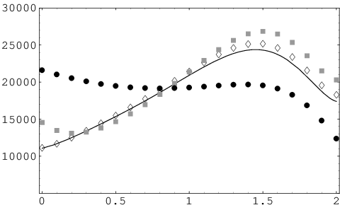
The next step was the computation of the amplitude with zero internal mass77 7 We thank Andre van Hameren for providing us with his program to compute massless one-loop scalar integrals., finding the results given in Fig. 1 and Fig. 2. It should be mentioned that our results are obtained algebraically, so there is no integration error involved.

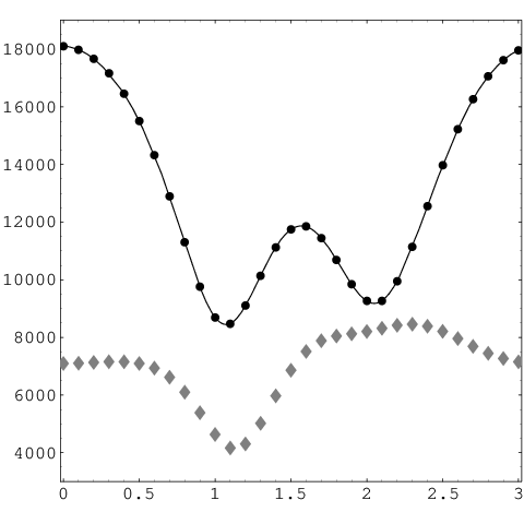
In Fig. 1, we reproduce the results presented by Nagy and Soper [19] and very recently also by Binoth et al.[20]. We employ the same values of the external momenta as in Fig. 5 of Ref. [19], namely the following selection of final state three-momenta :
| (45) |
After choosing the incoming photons such that they have momenta and along the -axis, we present in the plot the amplitude obtained by rotating the final states of angle about the -axis. This is done for both helicity configurations and . In the same plot also appears the analytic results for the configuration obtained by Mahlon [18]. In Fig. 2, we use a different set of external momenta. Starting from the following choice of :
| (46) |
we proceed as in the previous case. The results for the amplitudes are plotted in Fig. 2 for the helicity configurations and . It is known that the six-photons amplitude vanish for the helicity configurations and , we checked this result for both choices of the external momenta. Finally, using the external momenta of Eq. (4), we computed the amplitude introducing a non-zero mass for the fermions in the loop 88 8 We used here the scalar one-loop functions provided by FF[27].. The results are plotted in Fig. 3, for the three cases GeV, GeV and GeV.
The code we prepared for producing the results presented in this section is written in FORTRAN 90. Even if we did not spend too much effort in optimizations, it can compute about 3 phase-space points per second, when working in double precision. All figures in this section are actually produced by using double precision, but, to perform a realistic integration, we still need quadruple precision, that slows down the speed by about a factor 60. We are working in implementing the expansions presented in the previous section with the aim of being able to perform a stable integration over the full phase space, that is a “proof of concept” for any method.
5 Conclusions
Computing the massless QED amplitude for the reaction , although still unobserved experimentally, is a very good exercise for checking new methods to calculate one-loop virtual corrections. Such a process posses all complications typical of any multi-leg final state, for example a non trivial tensorial structure, but also keeps, at the same time, enough simplicity such that compact analytical formulas can still be used as a benchmark. However, it is oversimplified in two respects. Firstly, the amplitude it is completely massless. Secondly, the amplitude is cut constructible, namely does not contain any rational part.
In the most general case of one-loop calculations, the presence of both internal and external masses prevents from obtaining compact analytical expressions. Then one has to rely on other computational techniques. For example, it is known that cut-constructible amplitudes can be obtained through recursion relations. But, even then, the presence of rational parts usually requires a separate work.
For such reasons, it would be highly advisable to have a method not restricted to massless theories, in which moreover both cut-constructible and rational parts can be treated at the same time. Such a method has been introduced recently in Ref. [17] and, in this paper, we applied it to the computation of the six-photon amplitude in QED, giving also results for the case with massive fermions in the loop. We also showed in detail how the rational part of any -point one-loop amplitude is intimately connected with the form of the integrand of the amplitude. Once this integrand is numerically computable, cut-constructible and rational terms are easily obtained, at the same time, by solving the same system of linear equations. This is a peculiar property of our method, that we tested in the actual computation of the six-photon amplitude. In practice, we did not use the additional information on its cut-constructibility and verified only a-posteriori that the intermediate rational parts, coming from all pieces separately, drop out in the final sum.
Finally, we presented all relevant formulas needed to infer the rational parts from the integrand of any -point loop functions, in the renormalizable gauges.
In addition, we presented, by analyzing in detail the 2-point case, an idea to cure the numerical instabilities occurring at exceptional phase-space points, outlining a possible way to build up expansions around the zeroes of the Gram-determinants.
Having been able to apply our method to the computation of the massive six-photon amplitude, we are confident that our method can be successfully used for a systematic and efficient computation of one-loop amplitudes relevant at LHC and ILC.
Acknowledgments
We thank Andre van Hameren for numerical comparisons and Zoltan Nagy and Pierpaolo Mastrolia for interesting discussions. G.O. acknowledges the financial support of the ToK Program “ALGOTOOLS” (MTKD-CT-2004-014319). C.G.P’s and R.P.’s research was partially supported by the RTN European Programme MRTN-CT-2006-035505 (HEPTOOLS, Tools and Precision Calculations for Physics Discoveries at Colliders). The research of R.P. was also supported in part by MIUR under contract 2006020509_004.
Appendices
Appendix A Computing the extra-integrals
In this appendix, we compute the extra-integrals listed in Section 2. Since a contribution can only develop for non-negative dimensionality , the integrand in the Feynman parameter integral is always polynomial. First we decompose the integration as follows
| (47) |
then, after using Feynman parametrization and performing first the integral over and then that one over , one derives, for the extra-integrals of Eqs. (14)-(18)
| (48) |
where
| (49) |
In the following, we compute, as an illustrative example, the first three integrals of Eq. (A). The remaining two can be obtained analogously. We start by changing the integration variables as follows:
| . | |||||
| . | |||||
| (50) |
so that
| (51) |
from which one trivially obtains the first integral
| (52) |
To compute the second integral an integration over in needed. Since the integrand is symmetric when interchanging all , we concentrate on the coefficient of, say, . Since
| (53) | |||||
the final result reads
| (54) |
To compute the third integral we need to integrate over the product . Once again, given the symmetry of the problem, we can focus on the two contributions proportional to and . The first one gives
| (55) | |||||
and the second reads
| (56) | |||||
Summing up all of the possibilities one obtains
| (57) | |||||
Appendix B The general basis for the 2-point functions
In this appendix, we solve the problem of reconstructing the coefficients of the 2-point part of the integrand of any amplitude
| (58) |
by assuming at most quadratic in and . In particular also the case of vanishing is included. First, we introduce a massless arbitrary 4-vector , such that , that we use to rewrite in terms of two massless 4-vectors (we also take )
| (59) |
giving
| (60) |
Then, we introduce two additional independent massless 4-vectors defined as
| (61) |
for which one finds
| (62) |
and we decompose in the basis of , , and
| (63) |
so that takes the form
| (64) | |||||
Notice that, because of the identity
| (65) |
any term proportional to either contributes to the constant term or it is included in the terms we are neglecting 99 9 We suppose to determine them at a later stage of the calculation.. The same happens for the combination .
To be able to determine all of the coefficients appearing in Eq. (64), disentangling completely the contributions , we look for a that fulfill the requirement
| (66) |
For a written as in Eq. (63) this implies the system
| (67) |
where
| (68) |
It is convenient to introduce two classes of solutions. In the first class, that we call , we take fixed and choose . In the second class, that we call , we take fixed but choose . The coefficients , , , and can be obtained by evaluating Eq. (64) at the values
| (69) |
or
| (70) |
In the first case, the coefficients read
| (71) |
with
| (72) |
and where
| (73) |
In the second case, one obtains instead
| (74) |
with
| (75) |
and where
| (76) |
The reason why we have chosen two sets of solutions is that, in some special kinematical configurations, can vanish. Therefore, numerical stable solutions are obtained by taking and from Eq. (71), and and from Eq. (74), while is well defined in both cases.
The coefficients and can be determined, in terms of additional solutions of the kind and , by defining the combinations
| (77) |
as the two solutions of the system
The determinant of the matrix above is always different form zero, for non vanishing and , when , so that numerical inaccuracies never occur.
Finally, the two last coefficients and are determined, in terms of and , as solutions of the system
where
| (95) |
Once again one verifies that when, for example, the system never becomes singular.
References
- [1]
R. K. Ellis, W. T. Giele and G. Zanderighi,
JHEP 0605 (2006) 027
[arXiv:hep-ph/0602185];
R. Britto, B. Feng and P. Mastrolia, Phys. Rev. D 73 (2006) 105004 [arXiv:hep-ph/0602178];
C. F. Berger, Z. Bern, L. J. Dixon, D. Forde and D. A. Kosower, Phys. Rev. D 74 (2006) 036009 [arXiv:hep-ph/0604195];
Z. Bern, N. E. J. Bjerrum-Bohr, D. C. Dunbar and H. Ita, JHEP 0511 (2005) 027 [arXiv:hep-ph/0507019] ;
J. Bedford, A. Brandhuber, B. J. Spence and G. Travaglini, Nucl. Phys. B 712 (2005) 59 [arXiv:hep-th/0412108]. - [2]
See, for example, G. Belanger et al.,
Phys. Lett. B 576 (2003) 152
[arXiv:hep-ph/0309010];
A. Denner, S. Dittmaier, M. Roth and M. M. Weber, Nucl. Phys. B 680, 85 (2004) [arXiv:hep-ph/0309274]. - [3]
See, for example, A. Denner, S. Dittmaier, M. Roth and L. H. Wieders,
Nucl. Phys. B 724 (2005) 247
[arXiv:hep-ph/0505042] and
Phys. Lett. B 612 (2005) 223
[arXiv:hep-ph/0502063];
K. Kato et al., PoS HEP2005 (2006) 312. - [4] G. ’t Hooft and M. J. G. Veltman, Nucl. Phys. B 153 (1979) 365.
- [5] G. Passarino and M. J. G. Veltman, Nucl. Phys. B 160 (1979) 151.
- [6] A. Denner and S. Dittmaier, Nucl. Phys. B 734 (2006) 62 [arXiv:hep-ph/0509141].
- [7]
T. Binoth, J. P. Guillet and G. Heinrich,
Nucl. Phys. B 572 (2000) 361 [arXiv:hep-ph/9911342];
- [8]
A. Ferroglia, M. Passera, G. Passarino and S. Uccirati,
Nucl. Phys. B 650 (2003) 162
[arXiv:hep-ph/0209219];
W. T. Giele and E. W. N. Glover, arXiv:hep-ph/0402152;
D. E. Soper, Phys. Rev. D 62 (2000) 014009 [arXiv:hep-ph/9910292] and Phys. Rev. D 64 (2001) 034018 [arXiv:hep-ph/0103262];
Z. Nagy and D. E. Soper, JHEP 0309 (2003) 055 [arXiv:hep-ph/0308127]. - [9]
Z. Bern, L. J. Dixon, D. C. Dunbar and D. A. Kosower,
Nucl. Phys. B 435 (1995) 59
[arXiv:hep-ph/9409265];
Z. Bern, L. J. Dixon, D. C. Dunbar and D. A. Kosower, Nucl. Phys. B 425, 217 (1994). - [10] R. Britto, F. Cachazo and B. Feng, Nucl. Phys. B 725, 275 (2005).
- [11] E. Witten, Commun. Math. Phys. 252, 189 (2004); F. Cachazo, P. Svrcek and E. Witten, JHEP 0409 (2004) 006; A. Brandhuber, B. J. Spence and G. Travaglini, Nucl. Phys. B 706, 150 (2005); F. Cachazo, P. Svrcek and E. Witten, JHEP 0410, 074 (2004); I. Bena, Z. Bern, D. A. Kosower and R. Roiban, Phys. Rev. D 71, 106010 (2005).
- [12]
C. Anastasiou, R. Britto, B. Feng, Z. Kunszt and P. Mastrolia,
JHEP 0703 (2007) 111
[arXiv:hep-ph/0612277];
C. Anastasiou, R. Britto, B. Feng, Z. Kunszt and P. Mastrolia, Phys. Lett. B 645 (2007) 213 [arXiv:hep-ph/0609191];
D. Forde, arXiv:0704.1835 [hep-ph]. - [13] T. Binoth, J. P. Guillet, G. Heinrich, E. Pilon and C. Schubert, JHEP 0510 (2005) 015 [arXiv:hep-ph/0504267].
- [14] T. Binoth, J. P. Guillet and G. Heinrich, JHEP 0702 (2007) 013 [arXiv:hep-ph/0609054].
- [15]
Z. G. Xiao, G. Yang and C. J. Zhu,
Nucl. Phys. B 758 (2006) 1
[arXiv:hep-ph/0607015];
X. Su, Z. G. Xiao, G. Yang and C. J. Zhu, Nucl. Phys. B 758 (2006) 35 [arXiv:hep-ph/0607016]. - [16]
Z. Bern, L. J. Dixon and D. A. Kosower,
Phys. Rev. D 73 (2006) 065013 [arXiv:hep-ph/0507005];
S. D. Badger, E. W. N. Glover and K. Risager, arXiv:0704.3914 [hep-ph]. - [17] G. Ossola, C. G. Papadopoulos and R. Pittau, Nucl. Phys. B 763 (2007) 147 [arXiv:hep-ph/0609007].
- [18] G. Mahlon, Phys. Rev. D 49 (1994) 2197 [arXiv:hep-ph/9311213] and arXiv:hep-ph/9412350.
- [19] Z. Nagy and D. E. Soper, Phys. Rev. D 74 (2006) 093006 [arXiv:hep-ph/0610028].
- [20] T. Binoth, T. Gehrmann, G. Heinrich and P. Mastrolia, arXiv:hep-ph/0703311.
- [21] R. Pittau, Comput. Phys. Commun. 104, 23 (1997) [arXiv:hep-ph/9607309] and 111 (1998) 48 [arXiv:hep-ph/9712418].
- [22]
F. del Aguila and R. Pittau,
JHEP 0407 (2004) 017
[arXiv:hep-ph/0404120];
R. Pittau, arXiv:hep-ph/0406105. - [23] G. Devaraj and R. G. Stuart, Nucl. Phys. B 519 (1998) 483 [arXiv:hep-ph/9704308].
- [24] A. Denner and S. Dittmaier, Nucl. Phys. Proc. Suppl. 157 (2006) 53 [arXiv:hep-ph/0601085].
- [25] G. J. Gounaris, P. I. Porfyriadis and F. M. Renard, Eur. Phys. J. C 9 (1999) 673 [arXiv:hep-ph/9902230].
- [26] A. van Hameren, J. Vollinga and S. Weinzierl, Eur. Phys. J. C 41 (2005) 361 [arXiv:hep-ph/0502165].
- [27] G. J. van Oldenborgh, Comput. Phys. Commun. 66 (1991) 1.