Phase Transitions in the Coloring of Random Graphs
Abstract
We consider the problem of coloring the vertices of a large sparse random graph with a given number of colors so that no adjacent vertices have the same color. Using the cavity method, we present a detailed and systematic analytical study of the space of proper colorings (solutions).
We show that for a fixed number of colors and as the average vertex degree (number of constraints) increases, the set of solutions undergoes several phase transitions similar to those observed in the mean field theory of glasses. First, at the clustering transition, the entropically dominant part of the phase space decomposes into an exponential number of pure states so that beyond this transition a uniform sampling of solutions becomes hard. Afterward, the space of solutions condenses over a finite number of the largest states and consequently the total entropy of solutions becomes smaller than the annealed one. Another transition takes place when in all the entropically dominant states a finite fraction of nodes freezes so that each of these nodes is allowed a single color in all the solutions inside the state. Eventually, above the coloring threshold, no more solutions are available. We compute all the critical connectivities for Erdős-Rényi and regular random graphs and determine their asymptotic values for large number of colors.
Finally, we discuss the algorithmic consequences of our findings. We argue that the onset of computational hardness is not associated with the clustering transition and we suggest instead that the freezing transition might be the relevant phenomenon. We also discuss the performance of a simple local Walk-COL algorithm and of the belief propagation algorithm in the light of our results.
pacs
89.20.Ff, 75.10.Nr, 05.70.Fh, 02.70.-cI Introduction
Graph coloring is a famous yet basic problem in combinatorics. Given a graph and colors, the problem consists in coloring the vertices in such a way that no connected vertices have the same color GaJo. The celebrated four-colors theorem assures that this is always possible for planar graphs using only four colors 4colors. For general graphs, however, the problem can be extremely hard to solve and is known to be NP-complete NPcol, so that it is widely believed that no algorithm can decide in a polynomial time (with respect to the size of the graph) if a given arbitrary instance is colorable or not. Indeed, the problem is often taken as a benchmark for the evaluation of the performance of algorithms in computer science. It has also important practical application as timetabling, scheduling, register allocation in compilers or frequency assignment in mobile radios.
In this paper, we study colorings of sparse random graphs Bo; Janson. Random graphs are one of the most fundamental source of challenging problems in graph theory since the seminal work of Erdős and Rényi Erdos in 1959. Concerning the coloring problem, a crucial observation was made by focusing on typical instances drawn from the ensemble of random graphs with a given average vertex connectivity , as increases a threshold phenomenon is observed. Bellow a critical value a proper coloring of the graph with colors exists with a probability going to one in the large size limit, while beyond it does not exist in the same sense. This sharp transition also appears in other Constraint Satisfaction Problems (CSPs) such as the satisfiability of Boolean formulae GaJo. The existence of the sharp COLorable/UNCOLorable (COL/UNCOL) transition was partially 11 1 More precisely Friedgut proves the existence of a sharp threshold for a possibly size dependent sequence of thresholds, whose convergence is not proven. proven in Friedgut, and computing rigorously its precise location is a major open problem in graph theory. Many upper and lower bounds were established Lu; Nature; DuboisMandler; AchlioptasMoore03; AchlioptasRegular; Wormlad1; Wormlad2; Diaz for Erdős-Rényi and regular random graphs.
It was also observed empirically CKT91; Selman that deciding colorability becomes on average much harder near to the coloring threshold than far away from it. This onset of computational hardness cannot be explained only by the simple fact that near to the colorable threshold the number of proper colorings is small Hardness. Some progress in the theoretical understanding has been done by the analysis of search algorithms Hogg; Cocco. For the coloring problem, it was proven AcMo that a simple algorithm -colors almost surely in linear time random graphs of average connectivity for all (see AcMo for references on previous works). For 3-coloring the best algorithmic lower bound is AchlioptasMoore03. An important and interesting open question FrMcDi is the existence of an and of a polynomial algorithm which -colors almost surely a random graph of connectivity for arbitrary large .

The sharp coloring threshold and the onset of hardness in its vicinity has also triggered a lot of interest within the statistical physics community following the discovery of a close relation between constraint satisfaction problems and spin glasses NatureMonasson; Science. In physical terms, solving a CSP consists in finding groundstates of zero energy. The limit of infinitely large graphs corresponds to the thermodynamic limit. In the case of the coloring problem, for instance, one studies the zero temperature behavior of the anti-ferromagnetic Potts model WU. Using this correspondence, a powerful heuristic tool called the cavity method has been developed Science; MP99; MP03; MeZe; it allows an exact analytical study of the CSPs on sparse random graphs. Unfortunately, some pieces are still missing to make the cavity method a rigorous tool although many of its results were rigorously proven. The cavity method is equivalent to the famous replica method MPVkniha (and unfortunately for clarity, it has also inherited some of its notations, as we shall see).
The cavity method and the statistical physics approach have been used to study the -coloring of random graphs in Coloring; ColoringFlo; ColoringSaad. The coloring threshold was calculated Coloring, the self-consistency of the solution checked ColoringFlo and the large asymptotics of the coloring threshold computed ColoringFlo. These results are believed to be exact although proving their validity rigorously remains a major subject in the field. Nevertheless —as the results obtained for the random satisfiability problem MeZe; MeZeII; MPR03— they agree perfectly with rigorous mathematical bounds Lu; Nature; DuboisMandler; AchlioptasMoore03; AchlioptasRegular; Wormlad1; Wormlad2, and with numerical simulations. The coloring threshold is thus fairly well understood, at least at the level of cavity method.
A maybe more interesting outcome of the statistical physics analysis of the CSPs was the identification of a new transition which concerns the structure of the set of solutions, and that appears before the coloring threshold GiulioRemiMartin; Science; MeZe: while at low connectivities all solutions are in a single pure state (cluster) 22 2 In this paper we use the words ”cluster” and ”state” as synonyms., the set of solutions splits in an exponential number of different states (clusters) at a connectivity strictly smaller than . Roughly speaking, clusters are groups of near-by solutions that are in some sense disconnected from each other. Recently, the existence of the clustered phase was proven rigorously in some cases for the satisfiability problem Mora; Fede. A major step was made by applying the cavity equations on a single instance: this led to the development of a very efficient message-passing algorithm called Survey Propagation (SP) that was originally used for the satisfaction problem in Science and later adapted for the coloring problem in Coloring. Survey propagation allows one to find solutions of large random instances even in the clustered phase and very near to the coloring threshold.
Despite all this success, the cavity description of the clustered phase was not complete in many aspects, and a first improvement has been made with the introduction of a refined zero temperature cavity formalism that allows a more detailed description of the geometrical properties of the clusters ColoringMarc; OlivierThesis. We pursue in this direction and give for the first time a detailed characterization of the structure of the set of solutions. We observed in particular that the clustering threshold was not correctly computed, that other important transitions were overlooked and the global picture was mixed up. The corrected picture that we describe in this paper is the following: when the connectivity is increased, the set of solutions undergoes several phase transitions similar to those observed in mean field structural glasses (we sketch these successive transitions in fig. 1). First, the phase space of solutions decomposes into an exponential number of states which are entropically negligible with respect to one large cluster. Then, at the clustering threshold , even this large state decomposes into an exponential number of smaller states. Subsequently, above the condensation threshold , most of the solutions are found in a finite number of the largest states. Eventually, the connectivity is reached beyond which no more solutions exist. Another important transition, that we refer to as rigidity, takes place at when a finite fraction of frozen variables appears inside the dominant pure states (those containing almost all the solutions). All those transitions are sharp and we computed the values of the corresponding critical connectivities.
A nontrivial ergodicity breaking takes place at the clustering transition, in consequence uniform sampling of solutions becomes hard. On the other hand, clustering itself is not responsible for the hardness of finding a solution. Moreover, until the condensation transition many results obtained by neglecting the clustering effect are correct. In particular for all : i) the number of solutions is correctly given by the annealed entropy (and, for general CSP, by the replica symmetric entropy), and ii) simple message passing algorithm such as Belief Propagation (BP) Yedidia; BP-Pearl converges to a set of exact marginals (i.e. the probability that a given node takes a given color). In consequence we can use BP plus a decimation-like strategy to find proper colorings on a given graph. Finally we give some arguments to explain why the rigidity transition is a better candidate for the onset of computational hardness in finding solutions.
Our results are obtained within the one-step replica symmetry breaking approach, and we believe (and argue partially in section IV), that our results would not be modified by considering further steps of RSB (as opposed to previous conclusions ColoringFlo).
A shorter and partial version of our results, together with a study of similar issues in the satisfiability problem, was already published in US. We refer to THEM for a detailed discussion of the satisfiability problem. The paper is organized as follows: In section II, we present the model. In section III, we introduce the cavity formalism at the so-called replica symmetric level, and discuss in detail why and where this approach fails. In section IV we take into account the existence of clusters of solutions and employ the so called one-step replica-symmetry breaking formalism to describe the properties of clusters. The results for several ensembles of random graphs are then presented in section V. We finally discuss the algorithmic implications of our findings in section VI and conclude by a general discussion. Some appendixes with detailed computations complete the paper.
II The Model
II.1 Definition of the model
For the statistical physics analysis of the coloring problem ColoringSaad; Kanter; Coloring we consider a Potts WU spin model with anti-ferromagnetic interactions where each variable (spin, node, vertex) is in one of the different states (colors) . Consider a graph defined by its vertices and edges which connect pairs of vertices ; we write the Hamiltonian as
| (1) |
With this choice there is no energy contribution for neighbors with different colors, but a positive contribution otherwise. The ground state energy is thus zero if and only if the graph is -colorable. The Hamiltonian leads to a Gibbs measure GIBBS over configurations (where is the inverse temperature) :
| (2) |
In the zero temperature limit, where , this measure becomes uniform over all the proper colorings of the graph.
II.2 Ensembles of Random Graphs
We will consider ensembles of graphs that are given by a degree distribution . The required property of is that its parameters should not depend on the size of the graph. All the analytical results will concern only very large sparse graphs (). Provided the second and higher moments of do not diverge, such graphs are locally tree-like in this limit Bo; Janson. More precisely, call a -neighborhood of a node the set of nodes which are at distance at most from . For arbitrary but finite the -neighborhood is almost surely a tree graph when . This property is connected with the fact that the length of the shortest loops (up to a finite number of them) scales with the graph size as . We will consider the two following canonical degree distribution functions:
- (i)
Uniform degree distribution, , corresponding to the -regular random graphs, where every vertex has exactly neighbors.
- (ii)
Poissonian degree distribution, , corresponding to the Erdős and Rényi (ER) random graphs Erdos. A simple way to generate graphs with vertices from this ensemble is to consider that each link is present with probability . The binomial degree distribution converges to the Poissonian in the large size limit.
It will turn out that the cavity technics simplify considerably for the regular graphs. However, ER graphs have the advantage that their average connectivity is a real number that can be continuously tuned, which is obviously very convenient when one wants to study phase transitions. It is thus useful to introduce a third ensemble, which still has the computational advantage of regular graphs, but that at the same time gives more freedom to vary the connectivity:
- (iii)
bi-regular random graphs, where nodes with connectivity are all connected to nodes with connectivity , and vice-versa. There are thus two sets of nodes with degree distributions and .
Notice that these graphs are bipartite by definition and therefore have always a trivial -coloring which we will have to dismiss in the following. This can be easily done within the cavity formalism (it is equivalent to neglecting the ordered “crystal” phase in glass models GLASSFERRO).
In the first two cases, the parameter plays the role of the average connectivity, . In the cavity approach, a very important quantity is the excess degree distribution , i.e. the distribution of the number of neighbors, different from , of a vertex adjacent to a random edge :
| (3) |
This distribution remains Poissonian for Erdős-Rényi graphs, whereas the excess degree is equal to in the case of regular graphs. In the bi-regular case, there are two sets of nodes with excess degrees and .
III The cavity formalism at the replica symmetric level
We start by reviewing the replica symmetric (RS) version of the cavity method MP99; MP03 and its implications for the coloring problem. In the last part of the section we show when, and why, the RS approach fails.
III.1 The replica symmetric cavity equations
The coloring problem on a tree is solved exactly by an iterative method called the belief propagation algorithm BP-Pearl (note some boundary conditions have to be imposed, otherwise a tree is always 2-colorable) that is equivalent to the replica symmetric cavity method Yedidia. At this level, the method is in fact a classical tool in statistical physics to deal with that tree structure that dates back to the original ideas of Bethe, Peierls and Onsager BetheOnsager. It allows one to compute the marginal probabilities that a given node takes a given color and, in the language of statistical physics, observables like energy, entropy, average magnetization, etc. The applicability of the method goes however beyond tree graphs and we will discuss when it is correct for random locally tree-like graphs in section III.3.

Let us now describe the RS cavity equations. Denote the probability that the spin has color when the edge is not present and consider the iterative construction of a tree in fig. 2. The probability follows a recursion:
| (4) |
where is a normalization constant (the cavity partition sum) and the inverse temperature. The notation means the set of neighbors of except . The normalization is related to the free energy shift after the addition of the node and the edges around it, except , as
| (5) |
In the same way, the free energy shift after the addition of the node and all the edges around it is
| (6) |
The is at the same time the normalization of the total probability that a node takes color (the marginal of ):
| (7) |
The free energy shift after the addition of an edge is
| (8) |
The free energy density in the thermodynamic limit is then given by (see for instance MP99)
| (9) |
Note that this relation for the free energy is variational, i.e. that if one differentiates with respect to , then only the explicit dependence needs to be considered (see MP99 for details). The energy (the number of contradictions) and the corresponding entropy (the logarithm of the number of solutions with a given energy) densities can be then computed from the Legendre transform
| (10) |
were , and are intensive variables.
The learned reader will notice that in some previous works using the cavity method Coloring; ColoringFlo, these equations were often written for a different object than the probabilities . Instead, the so-called cavity magnetic fields and biases where considered. The two approaches are related via
| (11) |
Strictly speaking the are “cavity probabilities” while and are “cavity fields”, however are sometimes also referred to as cavity fields (or messages) in the literature, and the reader will thus forgive us if we do so.
Note that each of the two notations is suitable for performing the zero temperature limit in a different way: in the first one we fix the energy zero and we obtain the zero temperature BP recursion which gives the marginal probabilities for each variable, while in the second case, we obtain a simpler recursion called Warning Propagation (49) that deals with the energetic contributions but neglects the entropic ones MeZe; Coloring. This is the origin of the discrepancy between the RS results of refs. ColoringSaad and Coloring. As we shall see, the differences between these two limits will be an important point in the paper.
III.2 Average over the ensemble of graphs and the RS solution
To compute (quenched) averages of observables over the considered ensemble of random graphs given by the degree distribution we need to solve the self-consistent cavity functional equation
| (12) |
where is the distribution of the number of neighbors given that there is already one neighbor, and the function is given by eq.(4). Beware that here is a -components vector while we omit the vector notation to lighten the reading. This equation is quite complicated since the order parameter is nontrivial, but we can solve it numerically using the population dynamics method described in MP99; MP03.
Throughout this paper we will search only for the color symmetric functions , i.e. invariant under permutation of colors. Clearly with this assumption we might miss some solutions of (12). Consider for example colors and the ensemble of random bi-regular graphs. Since every bipartite graph is 2-colorable there are corresponding color asymmetric solutions for . For the ensemble of random graphs considered here, we later argue that this assumption is however justified.
Another important observation is that for regular graphs the equation (12) crucially simplifies: the solution factorizes Factorizes in the sense that the order parameter is the same for each edge. This is due to the fact that, locally, every edge in such a regular graph has the same environment. All edges are therefore equivalent and thus the distribution has to be a delta function. For the bi-regular graphs, the solution of (12) also factorizes, but the two sets of nodes of connectivity and (each of them being connected to the other) have to be considered separately.
It is immediate to observe that (i.e. each of the components of each cavity field equals ), is always a solution of (12). By analogy with magnetic systems we shall call this solution paramagnetic. Numerically, we do not find any other solution in the colorable phase. For regular random graphs the paramagnetic solution is actually the only factorized one. The number of proper colorings predicted by the RS approach is thus easy to compute. Since all messages are of the type , the free energy density simply reads
| (13) |
The entropy density at zero temperature thus follows
| (14) |
It coincides precisely with the annealed (first moment) entropy. We will see in the following that, surprisingly, the validity of this formula goes well beyond the RS phase (actually until the so-called condensation transition).
III.3 Validity conditions of the replica symmetric solution
We used the main assumption of the replica symmetric approach when we wrote eq. (4): we supposed that the cavity probabilities for the neighbors of the node are “sufficiently” independent in absence of the node , because only then the joint probability factorizes. This assumption would be true if the lattice were a tree with non-correlated boundary conditions, but loops, or correlations in the boundaries, may create correlations between the neighbors of node (in absence of ) and the RS cavity assumption might thus cease to be valid in a general graph. The aim here is to precise and quantify this statement both from a rigorous and heuristic point of view.
III.3.1 The Gibbs measure uniqueness condition
Proving rigorously the correctness of the RS cavity assumption for random graphs is a crucial step that has not yet been successfully overcome in most cases. The only success so far was obtained by proving a far too strong condition: the Gibbs measure uniqueness Aldous01; BG05; Jon; MSh06. Roughly speaking: the Gibbs measure (2) is unique if the behavior of a spin is totally independent from the boundary conditions (i.e. very distant spins) for any possible boundary conditions. More precisely, let us define colors of all the spins at distance at least from the spin . The Gibbs measure is unique if and only if the following condition holds for every (and in the limit )
| (15) |
where the average is over the ensemble of graphs. In BG05; Jon, it was proven that the Gibbs measure in the coloring problem on random regular graphs is unique only for graphs of degree . To the best of our knowledge, this has not been computed for Erdős-Rényi graphs (later in this section, we argue on the basis of a physical argument that it should be in this case).
III.3.2 The Gibbs measure extremality condition
In many cases, the RS approach is observed to be correct beyond the uniqueness threshold. It was thus suggested in MM05 (see also US) that the Gibbs measure extremality provides a proper criterion for the correctness of the replica symmetric assumption. Roughly speaking, the difference between uniqueness and extremality of a Gibbs measure is that although there may exist boundary conditions for which the spin is behaving differently than for others, such boundary conditions have a null measure if the extremality condition is fulfilled. Formally (and keeping the notations from the previous section), the extremality corresponds to
| (16) |
In mathematics the “extremal Gibbs measure” is often used as a synonym for a “pure state”. Recently, the authors of MM05 provided rigorous bounds for the Gibbs measure extremality of the coloring problem on trees.
There exist two heuristic equivalent approaches to check the extremality condition. In the first one, one studies the divergence of the so called “point-to-set” correlation length BiroliBouchaud; MS05. The second one is directly related to the cavity formalism: one should check for the existence of a nontrivial solution of the one-step replica symmetry breaking equations (1RSB) at (see section V). Both these analogies were remarked in MM05 and exploited in US. We will show in section V that the extremality condition ceases to be valid at the clustering threshold , beyond which the 1RSB formalism will be needed.
III.3.3 The local stability: a simple self-consistency check
A necessary, simple to compute but not sufficient, validity condition for the RS assumption is the non-divergence of the spin glass susceptibility (see for instance Rivoire). If it diverges, a spin glass transition occurs, and the replica symmetry has to be broken MPVkniha. The local stability analysis thus gives an upper bound to the Gibbs extremality condition, which remarkably coincides with the rigorous upper bound of KS66. This susceptibility is defined as
| (17) |
The connectivities above which it diverges at zero temperature can be computed exactly within the cavity formalism (we refer to appendix A for the derivation). It follows for regular and Erdős-Rényi graphs:
| (18) |
while the stability of the bi-regular graphs of connectivities is equivalent to regular graphs with .
Note that for regular and ER graphs the RS instability threshold is in the colorable phase only for . Indeed the 5-regular graphs are 3-colorable ColoringFlo (and rigorous results in Diaz; Wormlad2) and exactly critical since , and for ER graphs the COL/UNCOL transition appears at Coloring while . This means that the replica symmetry breaking transition appears continuously at the point so that above it the RS approach is not valid anymore. For all , however, the local stability point is found beyond the best upper bound on the coloring threshold for both regular and ER graphs. In this case, the extremality condition will not be violated by the continuous mechanism, but we will see that, instead, a discontinuous phase transition, as happens in mean field structural glasses, will take place.
Interestingly enough, a similar computation can be made for the ferromagnetic susceptibility (see again appendix A). It diverges at for regular graph and for Erdős-Rényi graphs. This divergence (called modulation instability in Rivoire) would announce the transition towards an anti-ferromagnetic ordering on a tree, which is however incompatible with the frustrating loops in a random graph (although such order might exist on the bi-regular graphs). This is precisely the solution we dismiss when considering only the color symmetric solution of (12). Note however that the presence of this instability shows that the problem ceases to a have a unique Gibbs state (although it is still extremal) as for some specific (and well-chosen) boundary conditions, an anti-ferromagnetic solution may appear. Indeed it coincides perfectly with the rigorous uniqueness condition for regular graph, and suggests strongly that the uniqueness threshold (or at least an upper bound) for Erdős-Rényi graphs is .
IV One-step replica symmetry breaking framework
So far we described the RS cavity method for coloring random graphs and explained that the extremality of the Gibbs measure gives a validity criterion. We now describe the one-step replica symmetry breaking cavity solution MP99; MP03. In this approach, the non-extremality of the Gibbs measure is cured, by decomposing it into several parts (pure states, clusters) in such a way that within each of the states the Gibbs measure becomes again extremal.
This decomposition has many elements/states, not just a finite numbers like the -states of the usual ferromagnetic Potts models. It is actually found that the number of pure states is growing exponentially with the size of the system. Let us define the state-entropy function —called the complexity— which is just the logarithm of the number of states with internal free energy density , i.e. . In the glass transition formalism, this complexity is usually referred to as the configurational entropy. Dealing with exponentially many pure states is obviously a nightmare for all known rigorous approaches to the thermodynamic limit. The heuristic cavity method overcomes this problem elegantly, as was shown originally in the seminal work of MP99; MP03.
Another very useful intuition about the 1RSB cavity method comes from the identification of states with the fixed points of the belief propagation equations (4). The goal is thus to compute the statistical properties of these fixed points. Each of the states is weighted by the corresponding free energy (9) to the power , where is just a parameter analogous to the inverse temperature (in the literature is often called the Parisi replica symmetry breaking parameter Parisi80; MPVkniha). The probability measure over states is then
| (19) |
where is just the normalization constant. To write the analog of the belief propagation equations we need to define the probability (distribution) of the fields . This can be obtained from those of incoming fields as
| (20) | |||||
The function is given by eq. (4) and the delta function ensures that the set of fields is a fixed point of the belief propagation (4). The re-weighting term takes into account the change of the free energy of a state after the addition of a cavity spin and its adjacent edges except , as defined in eq. (5). This term appears for the same reason as a Boltzmann factor in eq. (4): it ensures that the state is weighted by in the same way a configuration is weighted by in (2). Finally is a normalization constant. In the second line of (20) we introduced an abbreviation that will be used from now on to make the equations more easily readable. The notation POP comes from “population dynamics” which refers to the numerical method we use to solve eq. (20). The probability distribution can be represented numerically by a set of fields taken from , and then the probability measure becomes uniform sampling from this set, for more details see appendix D.
We define the “replicated free energy” and compute it in analogy with eq. (9) as
| (21) |
where
| (22) |
Putting together (19) and (21) we have
| (23) |
where the sum over is over all states (or BP fixed points). In the interpretation of Remi is the number of replicas of the system, thus the name “replicated free energy” for . Note that we are using the word “replica” only to refer to the established terminology as no replicas are needed within the cavity formalism. From the saddle point method, it follows that the Legendre transform of complexity function gives the replicated free energy
| (24) |
Notice that this equation is correct only in the highest order in the system size , i.e. in densities and at the thermodynamic limit. From the properties of the Legendre transform we have
| (25) |
Thus, from eq.(21), the free energy reads
| (26) |
When the parameter is equal to one (the number of replicas is actually one in the approach of Remi), then reduces to the usual free energy function considered in the RS approximation
| (27) |
where in the internal entropy density of the corresponding clusters and the total entropy density of the system.
IV.1 Analyzing the 1RSB equations
Combining (21) and (26) we can compute and for each value , that gives us implicitly . To compute the thermodynamic observables in the model we have to minimize the total free energy over such values of where the complexity is non-negative (so that the states exist in the thermodynamic limit). The minimum of the total free energy corresponds to a value of parameter and states with the free energy dominate the thermodynamics. Three different cases are then observed:
- a)
If there is only the trivial (replica symmetric) solution at , then the Gibbs measure (2) is extremal and the replica symmetric approach is correct. If at the same time a nontrivial solution exists for some , then the clusters corresponding to this solution have no influence on the thermodynamics.
- b)
If there is a nontrivial solution at with a positive complexity, then minimizes the total free energy. The system is in a clustered phase with an exponential number of dominating states.
- c)
If however the complexity is negative at , then the corresponding states are absent with probability one in the thermodynamic limit. Instead the total entropy is dominated by clusters corresponding to such that : the system is in a condensed phase. Note that the condition corresponds to the maximum of the replicated free energy (21).
The transitions between these cases are well known in structural glass phenomenology where they appear when the temperature is lowered REM; GLASSTHEORY. The transition from the paramagnetic phase to the clustered one is usually referred to as the dynamical transition MS06 or the clustering transition. It is not a true thermodynamic transition as the total free energy of the system at is still equal to the replica symmetric one (9) (see appendix C) and thus is an analytical function of connectivity. However, the phase space is broken into exponentially many components and, as a consequence, the dynamics fall out-of-equilibrium beyond this transition.
The second transition from the clustered to the condensed phase is, however, a genuine thermodynamic transition (the free energy has a discontinuity in the second derivative at ) and is called the replica symmetry breaking transition, or the static glass transition. At this point the measure condenses into few clusters, and we shall call it the condensation transition. In structural glasses, it corresponds to the well known Kauzmann transition Kauzmann. The sizes of the clusters in the condensed phase follow the so called Poisson-Dirichlet process which is discussed shortly in appendix B.
The procedure to compute the replicated free-energy (21) and the related observables was described above for a single large random graph. To compute the averages over the ensemble of random graphs, we need to solve an equation analogous to eq. (12)
| (28) |
where the functional is given by eq. (20). Solving this equation for a general ensemble of random graphs and a general parameter is a numerically quite tedious problem. In the population dynamics algorithm MP99; MP03 we need to deal with a population of populations of q-components fields. It is much more convenient to look at the ensemble of random regular graphs where a factorized solution must exists. Then we are left with only one functional equation (20).
Before discussing the zero temperature limit, we would like to point out that there exists another very important case in which eq. (28) simplifies. For , as first remarked and proved in MM05, when dealing with the problem of reconstruction on trees, the equations can be written (and numerically solved) in a much simpler way. We again refer to the appendix C for details. Especially for the Poissonian random graphs this simplification is very useful.
IV.2 Zero temperature limit
We now consider the zero temperature limit of the 1RSB equations (24)-(28) to study the coloring problem. In most of the previous works MP03; MeZe; Coloring the energetic zero temperature limit was employed. The limit of eq. (24) was taken in such a way that remains constant. The replicated free energy (24) then becomes
| (29) |
It is within this approach that the survey propagation (SP) algorithm was derived. The connectivity at which the complexity function becomes negative is the coloring threshold. Above this connectivity was used to compute the minimal number of violated constraints (the ground state energy). The reweighting in eq. (20) becomes , and when all the configurations with positive energy are forbidden.
In this paper we adopt the entropic zero temperature limit, suggested originally in ColoringMarc; OlivierThesis. The difference in the two approaches was already underlined in sec. III.1. We want to study the structure of proper colorings, i.e. the configurations of zero energy, and we thus fix the energy to zero. Then we obtain the entropy by considering and introduce a free entropy —or in replica term a “replicated entropy”— as . Eq. (24) then becomes
| (30) |
The belief propagation update (4) becomes
| (31) |
while the 1RSB equation (20) keeps the same expression (and thus the same computational complexity).
The partition sum in (2) becomes in this limit the number of proper colorings or solutions. The clusters are now sets of such solutions, and are weighted by their size to the power . The free entropy is then computed as
| (32) |
where and are given by eqs. (5) and (6). The analysis from the previous section is valid also for the entropic zero temperature limit. The information extracted from the number of clusters of a given size, , is one of the main results of this paper and will be discussed and interpreted in section V.
IV.3 The role of frozen variables
In this section we discuss the presence and the role of the frozen variables and explain the connection between the energetic and the entropic zero temperature limits. This allows us to revisit (and extend) the survey propagation equations. Remember that the components of the cavity field are the probabilities that the node takes the color when the constraint on the edge is not present. In the zero temperature limit we can classify them in two categories:
- (i)
A hard field corresponds to the case when all components of are zero except one, . Then only that color is allowed for the spin , in absence of edge .
- (ii)
A soft field corresponds to the case when more than one component of is nonzero. The variable is thus not frozen in absence of edge , and the colors of all the nonzero components are allowed.
This distinction is also meaningful for the full probabilities (4), if is a hard field then the variable is frozen. In the colorable region there cannot exist a finite fraction of frozen variables (even if we consider properly the permutational symmetry of colors) since by adding a link the connectivity changes by but the probability of becoming uncolorable would be finite. On the contrary, in the 1RSB picture, we observe that a finite fraction of variables can be frozen within a single cluster. In other words, in all the solutions that belong to this given cluster a finite fraction of variables can take one color only. By adding a link into the graph, the connectivity grows by , and there is a finite probability that a cluster with frozen variables disappears. The distinction between hard and soft fields is useful not only for the intuition about clusters, but also for the analysis of the cavity equations and it also leads to the survey propagation algorithm.
The distribution of fields over states (20) can be decomposed into the hard- and soft-field parts
| (33) |
where is the distribution of the soft fields and the normalization is .
Interestingly, the presence of frozen variables in the entropically dominating clusters is connected to the divergence of the size of average minimal rearrangement MS05; Guilhem_rear. Precisely, choose a random proper coloring and a random node in the graph. The average minimal rearrangement is the Hamming distance to the nearest solution in which node has a color different from averaged over the nodes , the proper colorings, and graphs in the ensemble.
Another interesting role of the frozen variables arises within the whitening procedure, introduced in ParisiWhit and studied, between others, for the satisfiability problem in Elitza; Riccardo. This procedure is equivalent to the warning propagation (WP) update (49) which we outlined in sec. III.1. Whitening is able to identify if a solution belongs to a cluster with frozen variables or not. Particularly, the result of the whitening is a set of hard cavity fields.
Since the survey propagation algorithm is computing statistics over the states that contain hard fields, then the solution found after decimating the survey propagation result should a priori also contain hard fields. However, recent works show that if one applies the whitening procedure starting from solutions found by SP on large graphs, whitening converges every time to the trivial fixed point (see detailed studies for K-SAT in Elitza; Riccardo). A possible solution to this apparent paradox is discussed in sec. VI.
IV.3.1 Hard fields in the simplest case,
Let us now consider the survey propagation equations originally derived in Coloring from the energetic zero temperature limit (29) when . For simplicity we will write them only for the 3-coloring. We consider the 1RSB cavity equation (20) for , then the reweighting factor is equal to zero when the arriving hard fields are contradictory, and equal to one otherwise. The update of probability that a field is frozen in direction is then written from eq.(20):
| (34) |
In the numerator there is a telescopic sum counting the probability that color and only color is not forbidden by the incoming fields. In the denominator the telescopic sum is counting the probability that there is at least one color which is not forbidden. If we do not want to actually find a proper coloring on a single graph but just to compute the replicated free energy/entropy, we can further simplify eq. (34) by imposing the color symmetry. Indeed, the probability that in a given state a field is hard in direction of a color has to be independent of (except which corresponds to a soft field). Then (34) becomes, now for general number of colors :
| (35) |
Note that since , the value corresponds to the point where the function has a zero slope. If a nontrivial solution of (35) exists, then is the maximum of the curve and is counting the total log-number of clusters of size , which is due to the exponential dependence, also the total log-number of all clusters, regardless their size. There are two points that we want to emphasize:
- •
Suppose that a nontrivial solution of (35) exists, i.e. many clusters exist and their number can be computed with the energetic zero temperature limit calculations. Then the clusters might be very small and contain very few solution in comparison to bigger less numerous clusters; or in comparison to a giant single cluster which might still exist. This situation cannot be decided by the energetic formalism that weights clusters equally independently of their size.
- •
Suppose, on contrary, that a nontrivial solution of (35) does not exist. It might still well be that many clusters exist, but the curve has no part with zero slope.
We will see that these two cases are actually observed. The energetic method, that can locate the coloring threshold and from which the survey propagation can be derived, is therefore not a good tool to study the clustering transition.
IV.3.2 Generalized survey propagation recursion
Let us compute how the fraction of hard fields evolves after one iteration of equation (20) at general . There are two steps in each iterations of (20). In the first step, iterates via eq. (35). In the second step we re-weight the fields. Writing the —unknown— distribution of the reweightings for the hard fields, one gets
| (36) |
A similar equation can formally be written for the soft fields
| (37) |
Writing explicitly the normalization , we finally obtain the generalized survey propagation equations:
| (38) |
In order to do this recursion, the only information needed is the ratio between between soft- and hard-field reweightings, which is in general difficult to compute since it depends on the full distribution of soft fields.
There are two cases where eq. (38) simplifies so that the hard-field recursion become independent from the soft-field distribution. The first case is, of course, then independently of the edge , and the equation reduces to the original SP. The second case arise for , where one can use the so-called reconstruction formalism and obtain again a closed set of equations. The computation is done in appendix C, and the SP equations at read
| (39) |
It would be interesting in the future to use eq. (38) in an algorithm to find proper graph colorings, as it has been done with the original SP equation Coloring. As an approximation one might also use a value independent of the edge , but different from one.
For the purpose of the present work, it is important to notice that it is also possible to use eq. (38) in the population dynamics to simplify the numerical evaluation of the 1RSB solution by separating the hard-field and the soft-field contributions. Indeed, it gives the exact density of hard fields provided the ratio is calculated, which is doable numerically (see appendix D). This allows us to monitor precisely the hard-field density and only the soft-field part is given by the population dynamics. This turns out to greatly improve the precision of the numerical solution of the cavity equations and to considerably fasten the code.
IV.3.3 The presence of frozen variables
A natural question is: “When are the hard fields present?” or more precisely: “When does eq. (38) have a nontrivial solution ?” First notice that in order to constrain a node into one color, one needs at least incoming fields that forbids all the other colors. It means that function defined in eq. (35) is identically zero for and might be non-zero only for , where is the number of incoming fields.
In the limit (which corresponds to ) eq. (38) gives if is positive, and if is zero. Updating eq. (38) on a given graph, from initial conditions everywhere, is equivalent to recursive removing of all the nodes of connectivity smaller than . This shows that the first nontrivial solution with hard fields exists if and only if the -core q_core of the graph is extensive. For regular graphs it is simply at connectivity while for Erdős-Rényi graphs these critical connectivities can be computed exactly and read, for small , , , q_core. Indeed we see that the first nontrivial solution to the 1RSB equation appears much before those of the original SP equation at .
On a regular graph, the equations further simplify as factorizes (is edge independent) and follows a simple self-consistent equation
| (40) |
This equation can be solved for every possible ratio so that for all , we can compute and plot the curve . We show the results in fig. 3 for different numbers of colors . On this plot, we observe that , as predicted, for . It then gets smaller for larger value of the ratio and, at a critical value , the solution disappears discontinuously and only the (trivial) solution exists. The values correspond to a critical value of . For all no solution containing frozen variables can exist.


IV.4 Validity conditions of the 1RSB solution
Now that we have discussed in detail the 1RSB formalism the next question is: “Is this approach correct?” To answer this question, one has to test if the Gibbs measure is extremal within the thermodynamically dominating pure states. This is equivalent to checking if the two-step Replica Symmetry Breaking (2RSB) solution is non trivial. Computing explicitly the 2RSB solution is however very complicated numerically, especially for Erdős-Rényi graphs. Instead, the local stability of the 1RSB solution towards 2RSB should be checked, in analogy with the RS stability in sec. III.3.3. It is indeed a usual feature in spin glass physics to observe that the 1RSB glass phase become unstable at low temperatures towards a more complex RSB phase and this phenomenon is called the Gardner transition Gardner.
To perform the stability analysis MR03; MPR03; ColoringFlo; Rivoire, one first writes the 2RSB recursion —where the order parameter is a distribution of distributions of fields on every edge — and then two types of 1RSB instabilities have to be considered depending on the way the 2RSB arises from the 1RSB solution. The first type of instability —called states aggregation— corresponds to while the second type —called states splitting— corresponds to . A complete stability analysis is left for future works, but it is worth to discuss the relevance of the results derived over the last few years MR03; MPR03; ColoringFlo.
The 1RSB stability was studied for the coloring problem in ColoringFlo but only for the energetic zero temperature limit (29). In this case the parameter is conjugated to the energy. The results derived in ColoringFlo —as well as those previously derived for other problems MR03; MPR03— thus concern only the clusters of sizes corresponding to at zero (for ) or at positive (for finite ) energy. The main result of ColoringFlo; MR03; MPR03 was that the 1RSB approach was stable in vicinity of the coloring threshold . As we shall see the clusters corresponding to are those dominating the total entropy at the coloring threshold and as a consequence its location is thus exact within the cavity approach. The states of the lowest energy (the ground states) in the uncolorable phase also correspond to , and thus the conclusions of ColoringFlo; MR03; MPR03 concerning the uncolorable phase are also correct. In particular, a Gardner transition towards further steps of RSB appears in the uncolorable phase beyond a connectivity denoted in ColoringFlo.
On the other hand in the colorable phase the stability of the entropically dominating clusters that correspond to should be investigated. Some more relevant information can be, however, already drawn from known results. It was indeed found that the 1RSB approach at is type I stable for all , and type II stable for all in vicinity of the coloring threshold. These results concerns the states of positive energy, but keeping in mind the interpretation of as a slope in diagram, we see that the clusters of zero energy corresponding to small but nonzero positive and zero temperature are also stable with respect to both types of stabilities. Near the colorable threshold, the value of which describes the dominating clusters is close to zero and as a consequence all the dominating clusters are 1RSB stable in vicinity of the coloring threshold. Far from the coloring threshold, the stability analysis of MPR03; ColoringFlo is irrelevant. In particular, the predictions of a full-RSB colorable phase made in ColoringFlo; MR03; MPR03 is not correct. Quite the contrary, our preliminary results indicate that all the dominating clusters are 1RSB stable for .
The coloring is however a special case as the clustering transition is continuous. Although the type II instability seems irrelevant in this case as well, we cannot at the moment dismiss a type I instability close to the clustering transition. Indeed the entropically relevant clusters correspond to values of close to one in this case, and it is simple to show that the clusters at are type I unstable in the case there is a continuous transition: this is because the type I stability is equivalent to the convergence of the 1RSB update on a single graph. Since for the averages of the 1RSB fields satisfy the RS belief propagation equations, and since we know from the RS stability analysis in section III.3.3 that those equations do not converge in the RS unstable region (i.e. for in 3-coloring of Erdős-Rényi graphs), it then follows that the 3-coloring is unstable against state aggregation at for all connectivities . Therefore, it is possible that the 1RSB result for 3-coloring are only approximative for what concerns the number and the structure of solutions close to the clustering transition (note that the critical values for the phase transition are however correct and do not depend on that). This, and related issues SUSY, will be hopefully clarified in future works.
To conclude, we believe that all the transition points we discuss in this paper (and those computed in the K-SAT problem in US) as well as the overall picture, are exact and would not be modified by considering further steps of replica symmetry breaking.
V The coloring of random graphs: cavity results
We now solve the 1RSB equations, discuss and interpret the results. We solve the equation (28) by the population dynamics technique, the technical difficulties and the precision of the method are discussed in appendix D. Let us stress at this point that the correctness of eq. (28) is guaranteed only in the limit of large graphs (), unfortunately the cavity method does not give us any direct hint about the finite graph-size corrections. We start by the results for the regular random graphs, then consider ensemble of bi-regular graphs and after that we turn towards Erdős-Rényi graphs. Finally, we discuss the limit of large number of colors.
V.1 Regular random graphs


Let us fix the number of colors , vary the connectivity, and identify successively all the transitions that we shall encounter. For the sake of the discussion, we choose as a typical example the 6-coloring and we discuss later in details the cases, for different number of colors, where some transitions are missing or are arriving in a different order. We solved the 1RSB equation (20) for regular graphs, where the distribution is the same for every edge (see appendix D) and plot the curves for we obtained doing so in fig. 4. We now describe the phase space of solutions when the connectivity is increased:
- 1)
At very low connectivities , only the paramagnetic RS solution is found at all . i.e. . The phase space is made of a single RS cluster.
- 2)
For larger connectivities , we saw in section IV.3.3 that the 1RSB equations start to have nontrivial solutions with hard fields in an interval . Interestingly, another nontrivial solution, without hard fields, can be found numerically in an interval , and we shall call this one the soft-field solution. As the connectivity increases, we find that increases while decreases, so that the gap where no nontrivial solution exists it getting continuously smaller.
However, there is no nontrivial solution at for connectivities smaller then (see fig. 4 for the example of the -coloring at ). This means that the Gibbs measure (2) is still extremal. In other words the large RS state still exists and is entropically dominant (its entropy (14) is noted by a circle in fig. 4). Despite the fact that an exponential number of clusters of solutions exist and that the SP equations converge to a nontrivial result, a random proper coloring will almost surely belong to the large RS cluster.
- 3)
If the connectivity is increased at and above the clustering threshold , a nontrivial solution with positive complexity is found at . In fig. 4, we see that this happens at for the regular -coloring. At this point, the RS Gibbs measure (2) ceases to be extremal and the single large RS cluster splits into exponentially numerous components. To cover almost all proper colorings we need to consider exponentially many clusters . The probability that two random proper colorings belong to the same cluster is going exponentially to zero with the system size. The connectivity is thus the true clustering (dynamic) transition. This is not, however, a thermodynamic phase transition because the 1RSB total entropy reduces to the RS entropy (14) at which is analytical in . Thus the RS approach gives a correct number of solution and correct marginals as long as the complexity function at is non-negative.
- 4)
For even larger connectivities , the complexity at becomes negative, e.g. for 6-coloring. It means that the clusters corresponding to are absent with probability one. The total entropy is then smaller than the RS/annealed one and is dominated by clusters corresponding to such that . The ordered weights of the entropically dominating clusters follow the Poisson-Dirichlet process (explained in appendix B). As a consequence, the probability that two random proper colorings belong to the same cluster is finite in the thermodynamic limit. Another way to describe the situation is that the entropy condenses into a finite number of clusters. This condensation is a true thermodynamic transition, since the total entropy is non-analytical at (there is a discontinuity in its second derivative with respect to connectivity). The condensation is analogous to the static (Kauzmann) glass transition observed in mean field models of glasses REM; GLASSTHEORY.
- 5)
For connectivities ( for -coloring) even the maximum of the complexity becomes negative. In this case proper colorings are absent with probability going to one exponentially fast with the size of the graph, and we are in the uncolorable phase.
It is useful to think of the growing connectivity as additions of the constraints into a fixed set of nodes. From this point of view the set of solutions which exists at connectivity gets smaller when new edges are introduced and the connectivity increased. This translates into the cartoon in the introduction (fig. 1) where all the successive transitions are represented. Finally, another important transition has to be considered:
- 6)
The presence or the absence of hard fields inside a given cluster is crucial: if a cluster contains only soft fields, then after the addition of a small but finite fraction of new constraints, its size will get smaller (or it will split). If, however, a cluster contains a finite fraction of frozen variable, then after adding a small but finite fraction of links the cluster will almost surely disappear.
Since the connectivities of regular graphs are integer numbers, we define the dynamical threshold as the smallest connectivity where a nontrivial 1RSB solution exists at , the condensation transition as the smallest connectivity where complexity at is negative, the smallest connectivity where hard fields are present at and the coloring threshold as the first uncolorable case. The scenario described here is observed for all cases of the regular ensemble, although, since connectivities are integer, the transitions are not very well separated at small . We summarize the results in table 1.
Note that for , the local RS stability discussed in section III.3.3 is irrelevant in the colorable regime. The only subtle case being for coloring of 5-regular graphs where the RS solution is only marginally stable, i.e. the spin glass correlation function goes to zero only algebraically instead of exponentially (from this point of view would correspond to the critical point well known in the second order phase transitions). More interesting cases will arise in the other ensembles of random graphs.
| q | ColoringFlo | MM05 | ColoringFlo | ||
|---|---|---|---|---|---|
| 3 | 5 | - | 6 | 6 | |
| 4 | 9 | 9 | - | 10 | 10 |
| 5 | 13 | 14 | 14 | 14 | 15 |
| 6 | 17 | 18 | 19 | 19 | 20 |
| 7 | 21 | 23 | - | 25 | 25 |
| 8 | 26 | 29 | 30 | 31 | 31 |
| 9 | 31 | 34 | 36 | 37 | 37 |
| 10 | 36 | 39 | 42 | 43 | 44 |
| 20 | 91 | 101 | 105 | 116 | 117 |
| q | ||||
|---|---|---|---|---|
| 5 | 3 | RS+ | 0.12 | 1.2(1) |
| 4 | 8 | RS | -0.03 | 3.4(1) |
| 4 | 9 | 1 | 0.41 | 0.41 |
| 5 | 12 | RS | -0.02 | 3.7(1) |
| 5 | 13 | RS | 0.20 | 2.0(1) |
| 5 | 14 | 0.50 | 0.90 | 0.90 |
| 6 | 16 | RS | -0.02 | 4.3(1) |
| 6 | 17 | RS | 0.05 | 3.2(1) |
| 6 | 18 | 1 | 0.40 | 0.40 |
| 6 | 19 | 0.92 | 0.96 | 0.96 |
| 7 | 21 | RS | 0.01 | 4.7(1) |
| 7 | 22 | RS | 0.17 | 3.2(1) |
| 7 | 23 | 1 | 0.60 | 0.60 |
| 7 | 24 | 1 | 0.95 | 0.95 |
V.2 Results for the bi-regular ensemble
The bi-regular ensemble allows us to fine-tune the connectivity while preserving the factorization of the 1RSB solution, which is crucial for the numerical precision. It is actually more correct to say that the solution is “bi-factorized”, as all the messages going from the nodes with connectivity to are the same and the other way around. The bi-regular ensemble allows us to describe with large precision two interesting cases, which reappear in the Erdős-Rényi ensemble and which are not present in the regular ensemble (again, due to the discrete nature of the connectivity). Let us remind here that bipartite graphs are always 2-colorable, but we consider only the color symmetric cavity solutions and that is why we get a nontrivial result from this ensemble.


In fig. 5, the left picture is the result for the complexity as a function of entropy for 4-coloring of 5-21-bi-regular graphs. The replica symmetric solution on this case is locally stable. We see clearly the gap between the hard-field and the soft-field solution, and yet we are already beyond the clustering transition ; actually the system is in the condensed phase. This example is similar to what happens for the 4-coloring of Erdős-Rényi graphs.
The second interesting case, the right hand side of fig. 5, is given by the results for for the 4-coloring of 4--bi-regular graphs, which are RS unstable for . Both the clustering and the condensation transitions coincide with the RS instability . The survey propagation equations have a nontrivial solution starting from . The rigidity transition is at . Finally the coloring threshold is . Qualitatively, the results for this 4--bi-regular ensemble are the same as those for the 3-coloring of Erdős-Rényi random graphs.
We see that for the gap between the hard-field (full line) and soft-field (dotted line) solution exists. For there is a non-physical nontrivial soft-field solution, the convex part of the line in the figure, zoomed in the inset. It means that for we actually can find two solutions depending if we start or not with a population containing enough hard fields. The unphysical branch survives even when the gap closes, see the example of in the figure.
We would like to stress at this point the enormous similarity of the soft-field part of the curve to the one in fig. 4 in ref. GiulioRemiMartin. Actually the variational results of GiulioRemiMartin should be very precise and relevant near to the continuous clustering transition (this is also case for the 3-coloring of Erdős-Rényi graphs or for 3-SAT).
V.3 Results for Erdős-Rényi random graphs
For Erdős-Rényi random graphs obtaining the solution of eq. (28) is computationally more involved as the solution is no longer factorized. In the population dynamics a population of populations has to be updated, which is numerically possible only for small populations, and so one has to be careful that the finite population-size corrections are small enough, see details in appendix D. However, all the computations can be done with the same computational complexity as for the regular graphs for , the energetic zero temperature limit (section IV.3.1), and for (appendix C). That is enough to obtain the SP, clustering, condensation and COL/UNCOL transitions (from which the first and last one was computed in Coloring). We can also compute exactly when hard fields appear for , eq. (72), this transition is further studied in Guilhem_rear. Finally, using the generalized survey propagation equation introduced in section IV.3.2, the rigidity transition can be computed quite precisely.
V.3.1 The general case for , discontinuous clustering transition
The phase transitions in -coloring of random Erdős-Rényi graphs for are qualitatively identical to those discussed in the case of random regular graphs. We plot the results for the total entropy (number of solutions) and complexity (number of clusters which dominate the entropy) in the and coloring in fig. 6.
At the clustering transition the complexity becomes discontinuously positive, the large RS cluster suddenly splits in an exponential number of smaller ones. The total entropy is given by the RS formula (14) up to the condensation transition . At the condensation transition the complexity of the dominating clusters becomes zero, the total entropy is given by the point where . The function is non-analytical at the point , it has a discontinuity in the second derivative. At the coloring threshold all the clusters of solutions disappear, note, however, that the total entropy of the last existing clusters is strictly positive (about a half of the total entropy at the condensation transition). That means that the COL/UNCOL transition is not only sharp but also discontinuous in terms of entropy of solutions. Note that the positive entropy has two contributions: the trivial and smaller one coming from presence of leaves and other small subgraphs, and the nontrivial and more important one connected with the fact, that the ground state entropy is positive, even in the uncolorable phase or for the random regular graphs.
Finally we located the rigidity transition, when frozen variables appears in the dominating clusters. For this transition appears in the condensed phase. As the number of colors grows it approaches the clustering transition. All the four critical values , , and are summarized in table 2, values of and are given for comparison.


| q | ||||||
|---|---|---|---|---|---|---|
| 3 | 4 | 4.66(1) | 4 | 4.687(2) | 4.42(1) | 4.911 |
| 4 | 8.353(3) | 8.83(2) | 8.46(1) | 8.901(2) | 8.09(1) | 9.267 |
| 5 | 12.837(3) | 13.55(2) | 13.23(1) | 13.669(2) | 12.11(2) | 14.036 |
| 6 | 17.645(5) | 18.68(2) | 18.44(1) | 18.880(2) | 16.42(2) | 19.112 |
| 7 | 22.705(5) | 24.16(2) | 24.01(1) | 24.455(5) | 20.97(2) | 24.435 |
| 8 | 27.95(5) | 29.93(3) | 29.90(1) | 30.335(5) | 25.71(2) | 29.960 |
| 9 | 33.45(5) | 35.658 | 36.08(5) | 36.490(5) | 30.62(2) | 35.658 |
| 10 | 39.0(1) | 41.508 | 42.50(5) | 42.93(1) | 35.69(3) | 41.508 |
V.3.2 The special case of coloring, continuous clustering transition
The only case which is left to be discussed is the 3-coloring of Erdős-Rényi graphs. It is different from because the replica symmetric solution is locally unstable in the colorable phase (see section III.3.3). The extremality condition underlying the RS assumption ceases to be valid because of the mechanism discussed in section III.3.3, with a divergence of the spin glass correlation length: the main difference with the previous cases is therefore that the clustering transition is continuous and coincide with the condensation transition.
However, the phenomenology does not differ too much from the other cases: ; the phase where the entropy is dominated by exponential number of states is thus missing and the complexity corresponding to is always negative (see fig. 7 left together with the dependence of the total entropy on the connectivity). Note that the curves for the 3-coloring have been already studied in ColoringMarc; OlivierThesis where the authors considered however only the range of connectivities .
All the results derived for the 4-coloring of 4--bi-regular bipartite graphs are quantitatively valid also here. We are thus not surprised by the fact that in interval the survey propagation algorithm gives us a trivial result: simply the maximum of the curve does not exist yet there is no nontrivial solution at . Yet, the entropy is dominated by finite number of largest clusters which do not contain hard fields. The two solutions (hard-field and soft-field) join at a connectivity around . Finally at the hard fields arrive to the dominating states (and in consequence to all others).


V.3.3 The overlap structure
We now give some results about the overlap structure in the random coloring to elaborate the intuition about clusters. First, consider marginal probabilities within a cluster . Note that due to the color symmetry there exist another clusters different only in the permutation of colors. We define the intra-cluster overlap of two solutions (averaged over states) as
| (41) |
In the paramagnetic phase , otherwise we have to compute it from the fixed point of equation (20). The overlap between two solutions which lie in two clusters, which differ just by permutation of colors is
| (42) |
where is the number of fixed positions in the permutation (in particular , and ). In fig. 8 we show the overlap structure for 3- and 4-coloring. The probabilities that two random solutions have one of the overlaps can be computed from the Poisson-Dirichlet process described in appendix B, in fact this is not a self-averaging quantity MPVkniha.


V.4 Large q Asymptotics
We give here the exact analytical large expansion of the previous results. In the asymptotic computations the regular and Erdős-Rényi ensembles are equivalent (the corrections are of smaller order in that the orders we give). We refer to the appendix E for the explicit derivation of the formulae.
At large a first set of transitions arises for connectivities scaling as :
| (43) | |||||
| (44) |
was already computed in ColoringFlo and is the rigidity transition. The clustering transition has to appear before the rigidity one . For all the finite cases we looked at, was between and .
A second set of transitions arises for connectivities scaling as :
| (45) | |||||
| (46) |
The condensation thus appears very close the COL/UNCOL transition and both are very far from the clustering and rigidity transitions (those are on a half way in the phase diagram).
We show also in appendix E that for connectivity , one has
| (47) | |||||
| (48) |
Since the RS free energy is correct until , which differers just by constant from , that means that for all connectivities bellow the number of solutions is correctly given by the replica symmetric entropy (14). Indeed, the value can be obtain by a large expansion of eq. (14).
In fig. 9 we plot the complexity of dominating clusters , the total entropy , and the physical value of as a function of connectivity . Note that the properly scaled values of the total number of solutions at and , and the values , themselves, are already very close to those at (see figs. 6 and fig. 7 left). The closeness is particularly striking for the values for and (see fig. 7 right).
These formulae show that in the large limit, near to the coloring threshold, it is the number of clusters which change with connectivity (i.e. ), and not their internal entropy (size). In the leading order, adding constraints near to the COL/UNCOL transition thus destroys clusters of solutions, but do not make them smaller: this is due to the fact that these clusters are dominated by frozen variables so that adding a link kills them most of the time. We also computed the entropy value at the condensation transition, and found . The entropy of the last cluster (exactly at the COL/UNCOL transition) is .


VI Algorithmic consequences
In this section we give some algorithmic consequences of our findings. First, we discuss the whitening procedure. We then introduce a random walk algorithm adapted from the Walk-SAT strategy and study its performance. We show in particular that the clustering/dynamical transition does not correspond to the onset of hardness in the problem and argue that it is instead the rigidity transition. Finally, we discuss the performance of the belief propagation algorithm in counting and finding solutions, and show that is works much better than previously anticipated.
VI.1 The whitening procedure
The whitening procedure as introduced in ParisiWhit can distinguish between solutions which belong to a cluster containing hard fields and those which do not. Generally whitening is equivalent to the warning propagation (version of belief propagation which distinguish only if a field is hard or not). Warning propagation for coloring was derived in Coloring. Let us call the hard field in the direction of the first color, i.e. in absence of node the node takes only the first color in all the colorings belonging to the cluster in consideration, and similarly for other colors. Denote if is not frozen in the cluster, we say that the oriented edge is then “white”. The update for ’s follows from (4)
| (49) |
To see if a solution belongs to a cluster with frozen variables or not we initialize warning propagation with , and update iteratively according to (49) until a fixed point is reached (the update every time converge, because starting from a solution we are only adding white edges). In the fixed point or all edges are white, then the solution does not belong to a frozen cluster, or some of the edges stay colored (non-white), then the solution belongs to a frozen cluster. Note that in the K-SAT problem (but not in general), whitening is equivalent to a more intuitive procedure, where the directed edged are not considered Elitza; Riccardo.
We wish to offer here an explanation of a paradox observed in Elitza; Riccardo. The SP algorithm gives information on the frozen variables in the most numerous clusters (). Yet, the solutions which are found by the standard implementation (decimation and SP plus Walk-SAT) do not belong to clusters with frozen variables, since they always give a trivial whitening result (all directed edges are white)Elitza; Riccardo. We suggest that the decimation strategy drives the system towards a solution belonging to a large cluster, which does not contain frozen variables. In this case, it is logical that the result of the whitening is trivial, as it is observed. We believe this is reason why no nontrivial whitenings are observed so far in the study of the K-SAT problem on large graphs.
Note that beyond the rigidity transition this argument does not work anymore, since there all the clusters (for all such that ) contain frozen variables. More precisely, for we could in principle end up in soft-clusters even beyond the rigidity transition (since that one concerns only the dominant states), if this is possible is let for further investigation. Interestingly, in the coloring problem we have not been able to find solutions beyond the rigidity transition even with survey propagation algorithm (compare with the performance of SP in Coloring). Further, more systematic, investigations have to be done about these issues, employing other strategies for the use of the survey propagation equations (for example the reinforcement reinforcement).
VI.2 A Walk-COL algorithm to color random graph
In this paper, we have computed the correct clustering transition for the random coloring problem. Beyond this transition, Monte Carlo algorithms are proven not to reach equilibrium as their time of equilibration diverges MS05; MS06. It was often claimed, or assumed, that this point corresponds to the onset of hardness of the problem. However, the fact that the physical dynamics does not equilibrate just means that the complete set of solutions will not be correctly sampled —indeed Monte-Carlo experiments clearly display slow relaxation MonteCarlo— but not that no solutions can be eventually found. This simple fact explains the results of ColoringSaad where a simple annealing procedure was shown to 3-color a ER graph beyond .
In this section, we use a local search strategy which does not satisfy the detailed balance condition. Therefore, we do not expect to be able to find typical solutions, however it might be possible to find some solutions to the problem. The Walk-COL algorithm 33 3 A slightly different adaptation, closer to walksat, was performed few years ago by Andrea Pagnani and Martin Weigt (private communication). is a simple adaptation of the celebrated Walk-SAT walksat. More precisely, we adapted the method designed for satisfiability in John. Given a graph, and starting from an initial random configuration, we recursively apply the following procedure:
- 1)
Choose at random a spin which is not satisfied (i.e. at least one of its neighbors has the same color).
- 2)
Change randomly its color. Accept this change with probability one if the number of unsatisfied spin has been lowered, otherwise accept it with probability .
- 3)
If there still are unsatisfied nodes, go to step 1) unless the maximum running time is reached
The probability has to be tuned in each different case for a better efficiency of the algorithm. Typically, values between give good results. We shall now briefly discuss the performance of the algorithm, to illustrate the two following points: (a) When the phase space is RS, we observe that Walk-COL finds a solution in linear time. (b) Even in the “complex” phase for , the algorithm can find in some cases solutions in linear time.
Concerning the first point, we tested the algorithm in the RS phase of regular random graphs for . In all these cases, we were able to color in linear time all the graphs of connectivities that correspond to a replica symmetric solution. In particular, the cases , , , , are found to be colorable with the Walk-COL algorithm even if a nontrivial solution to the SP equations exists.
Concerning the second point, we considered the and coloring of Erdős-Rényi random graphs. The results are shown in fig. 10 where the percentage of unsatisfied spins versus the number of attempted flips (averaged over different realizations) divided by is plotted. We observe that the curves corresponding to different values of superpose quite well (and that actually the results for are systematically lower than those for ) so that an estimation of the time needed to color a graph can be obtained. The connectivities of these graphs are beyond the dynamical transition ( for 3-coloring and for 4-coloring). It would be interesting to systematically test Walk-COL, as it has been done for Walk-SAT in John, to derive the precise connectivity at which it ceases to be linear.


Already these results show that the dynamical transition is not a problem for the algorithms. This can also be observed in a number of numerical experiments for the satisfiability walksat_whitening; John and the coloring Jorge; Stefan problems.
We believe, however, that the rigidity transition plays a fundamental role for the average computational complexity. A first argument for this is that, for large graphs, it seems that all the known algorithms are only able to find solutions with a trivial whitening, i.e. solutions that belong to clusters without hard fields. Beyond the rigidity transition however, the clusters without hard fields become very rare (in the sense that the dominating clusters and all the smaller, more numerous ones, contain hard fields). For maybe the connectivity where hard fields appear in clusters corresponding to , should be considered. This suggests that the known algorithms will not be able to find a solution beyond this point.
A second argument is the following: local search algorithms are either attracted into a solution or stucked in a metastable state. These metastable states, in order to be able to trap the dynamics, have to contain a finite fraction of hard fields. Given an algorithm, determining which of these two situations happens is not only a question of existence of states, but also a question of basins of attraction and a theoretical analysis of such basins is a very difficult task so that the precise analysis of the behavior of local algorithms remains a hard problem. However, the metastable states are known, from the cavity formalism, to be much more numerous than the zero-energy states. Moreover the basin of attraction of a zero-energy state that contains hard fields does not probably differ much from those of the metastable state (while, on the other hand, the basin of attraction of a zero-energy state which does not contain hard fields might be slightly different and arguably relatively larger). It thus seems to us reasonable that local algorithms will get trapped by the metastable states beyond the rigidity transition.
A similar conclusion was reached recently in Jorge where the recursive implementation of the Walk-COL algorithm was studied and found to be somehow simpler to analyze. Again the strategy was found to be efficient (with linear time with respect to the size of the graph) beyond but bellow . The precise algorithmic implications of the rigidity transition thus require further investigation, maybe in the lines of walksat_whitening; Jorge.
VI.3 A belief propagation algorithm to color random graph
Another consequence of our results, that we already discussed shortly in US, is that the standard belief propagation (BP) algorithm gives correct marginals until the condensation transition. It is actually a simple algebraic fact that the 1RSB approach at gives the same results for the marginals (average probabilities over all clusters) as the simple RS approach (see appendix C). Moreover the log-number of solutions in clusters corresponding to is also equal to the RS one. This suggests to use the BP marginals (as was already suggested in BP-Pearl) and a decimation procedure to find proper colorings. Compared with the SP algorithm which has computational complexity proportional to (factorial) the BP is only . We have seen moreover that for large numbers of colors, the condensation point is very close to the COL/UNCOL transition, so that BP could be used in a large interval of connectivities.
As a simple application, we tested how the straightforward implementation of the BP algorithm plus decimation allows one to find solutions of and coloring of random Erdős-Rényi graphs. Note that in the coloring the clustered but not condensed phase is missing, so the argumentation above does not concern this case. The algorithm works by iterating the following procedure:
- (i)
Run BP on the graph for a given number of iterations.
- (ii)
Consider the most biased variable, and color it with its most probable color.
Two problems have to be mentioned. The first one is rather trivial: since at the beginning all colors are symmetric, the first color had to be put at random. The second one is more serious and concerns the convergence of BP. Indeed, we saw that there is local instability in the BP (replica symmetric) equations at connectivity for the coloring of random graphs, so that the BP equations do not converge. This seems to be a problem restricted to the coloring, but even in the case of or more coloring, the BP equations do not converge on the decimated graph when a finite fraction (typically few percent) of variables is fixed. The reason or that is to be understood.
Nevertheless, since we merely want to design an effective tool to solve the coloring problem, we choose to avoid this problem by fixing the number of iteration at each step and thus ignore the non-convergence. We tried the method on both the and coloring and obtained unexpectedly good results. We used the following protocol in the code: We first try to find a solution with . If we do not succeed, we restart with and once more with . We tried that on different samples for different connectivities. The probability to find a proper coloring with these conditions is shown in fig.11.


We thus observe that the BP strategy is able to find solutions, even beyond the condensation transition. This shows clearly that the decimation procedure is a nontrivial one, and that the problem is not really hard in that region of connectivities. Note that the SP algorithm plus decimation has been shown to work in the coloring very well until about Coloring: our results are thus very close to those obtained using SP. This rises again the question of the rigidity transition , which might also be problematic for the decimated survey propagation solver.
VII Conclusions
Let us summarize the results. They are perhaps best illustrated looking back to the cartoon in fig. 1, where the importance of the size of clusters is evidenced. We find that the set of solutions of the -coloring problem undergoes the following transitions as the connectivity is increased:
- (i)
At low connectivity, , many clusters might exist but they are very small and the measure over the set of solutions is dominated by the single giant cluster described by the replica symmetric approach.
- (ii)
Only at the dynamical transition the giant cluster decomposes abruptly into an exponentially large number of clusters (pure states). For connectivities , the measure is dominated by an exponential number of clusters. Yet, the total number of solutions is given by the replica symmetric entropy (14), and the marginals are given by the fixed point of the replica symmetric equations (belief propagation) (4). Starting from this transition the uniform sampling of solution becomes hard.
- (iii)
At connectivity the set of solutions undergoes a condensation transition, similar to the one appearing in mean field spin glasses. In the condensed phase the measure is dominated by finite number of the largest clusters. The total entropy is strictly smaller than the replica symmetric one and has a discontinuity in the second derivative at .
- (iv)
When connectivity is reached, no more clusters exist: this is the COL/UNCOL transition. Note that the entropy of last existing clusters is strictly positive, and not given only by the contribution of the isolated nodes, leaves and other small subgraphs, the COL/UNCOL transition is thus discontinuous in entropy.
.
This picture is very similar to the well-known scenario of the glass transition in temperature, with the dynamical and glass (Kauzmann) transition GLASSTHEORY. In some cases, the main one being the 3-coloring of Erdős-Rényi graphs, the clustering and the condensation transition merge and a continuous transition take place at , which then coincide with the local instability of the replica symmetric solution. Interestingly the variational approach of GiulioRemiMartin is very precise near to the continuous clustering transition. Since the 3-SAT problem behaves in the same manner, this solves the apparent contradictions between the results of GiulioRemiMartin and Science.
In addition to the transitions describing the organization of clusters, another important phenomenon concerning the internal structure of clusters takes place. A finite fraction of frozen variables can appear in the clusters (a frozen variable takes the same color in all the solutions that belong to the cluster). We found that the fraction of such variables in each cluster undergoes a first order transition and jumps from zero to a finite fraction at a connectivity that depends on the size of the cluster. In particular:
- (v)
There exists a critical connectivity (rigidity/freezing) at which the thermodynamically relevant clusters —those that dominate the Gibbs measure— start to contain a finite fraction of frozen variables.
The results above were obtained within the 1RSB scheme, but should not change when considering further steps of RSB (an exception might be the 3-coloring near to the clustering transition).
We discussed some algorithmic consequences of these transitions. First, the belief propagation algorithm is efficient in counting solution and estimating marginals until the condensation transition. More interestingly, it can also be used, just like survey propagation, together with a decimation procedure in order to find solutions as we numerically demonstrated. Secondly, the dynamical transition is not the one at which simple algorithms fail as we illustrated using the Walk-COL strategy. For the 3-coloring of ER graph, there is even a rigorous proof of algorithmic performance beyond and until AchlioptasMoore03. We argued that, instead, the rigidity phenomenon is responsible for the onset of computational hardness. This is a major point that we hope to see more investigated in the future.
Our study opens a way to many new and promising investigations and developments. For instance, we wrote the equivalent of the survey propagation equations for general value of , which has a particularly simple form for (39). It would be interesting to use these equations to find solutions. The behavior at finite temperature and the performance of the annealing procedure are also of interest. It would furthermore be interesting to re-discuss other finite connectivity spin glass models like for instance the lattice glass models Rivoire in the light of our findings. The stability towards more steps of replica symmetry breaking, or the super-symmetric approach SUSY, should be further investigated. Finally, it would be interesting to combine the entropic and energetic approach to investigate the frozen variables in the meta-stable states. We hope that our results will stimulate the activity in these lines of thoughts.
Acknowledgements.
We thank Jorge Kurchan, Marc Mézard, Andrea Montanari, Federico Ricci-Tersenghi, Guilhem Semerjian and Riccardo Zecchina for cheerful and very fruitful discussions concerning these issues. The numerical computations were done on the cluster EVERGROW (EU consortium FP6 IST) at LPTMS, Orsay, and on the cluster DALTON at ESPCI, Paris. This work has been partially supported by EVERGROW (EU consortium FP6 IST).Appendix A Stability of the paramagnetic solution
In this appendix, we show how to compute the stability of the paramagnetic solution towards the continuous appearance of a 1RSB solution. This happens, as usual for continuous transition, when the spin glass correlation length, or equivalently, the spin glass susceptibility, diverges. Obviously, the presence of the diverging correlation length invalidate the premise of the RS cavity method. Recall that the spin glass susceptibility is defined as
| (50) |
and can be rewritten for the present purpose as
| (51) |
where we consider the average over graphs, in the thermodynamic limit, where spins and are at distance . The factor stands for the average number of neighbors at distance , when . Assuming that the limit for large of the summands in (51) exists (with the limit performed first), we relate it to the stability parameter:
| (52) |
Then the series in (51) is essentially geometric, and converges if and only if .
Using the fluctuation-dissipation theorem we relate the correlation to the variation of magnetization in , caused by an infinitesimal field in . Finally, using the fact that we perform the large- limit first, the variation above is dominated by the direct influence through the length- path between the two nodes, and this induces a “chain” relation: if the path involves the nodes we have
| (53) |
The stability parameter of the paramagnetic solution of the cavity equations towards small perturbations can be computed from the following Jacobian
| (54) |
which gives the infinitesimal probability that a change in the input probability will change the output probability . The index RS says that the expression has to be evaluated at the RS paramagnetic solution.
This matrix has only two different entries, all the diagonal elements are equal, and all the non-diagonal elements are also equal. As an immediate consequence all Jacobians commute and are thus simultaneously diagonalizable so that it will be sufficient to study the effect after one cavity iteration (one step in the chain). The matrix has only two distinct eigenvalues,
| (55) |
The second eigenvalue corresponds to the homogeneous eigenvector and describes a fluctuation changing all by the same amount, and maintains the color symmetry. It is thus not likely to be the relevant one and we will see that indeed . The first eigenvalue, however, is -fold degenerate and its eigenvectors are spanned by . The corresponding fluctuations explicitly break the color symmetry, and are in fact the critical ones. Using the cavity recursion (4), the two derivatives simply read
| (56) |
so that the values of the two eigenvalues evaluated at the RS solution, where all are equal to , are
| (57) |
The stability parameter (52) is thus and the critical temperatures bellow which the instability sets in are
| (58) |
For regular and Erdős-Rényi graphs respectively. Thus at zero temperature the critical connectivities reads
| (59) |
These results coincide perfectly with the numerical simulations of the cavity recursion of ColoringSaad. The analytical expressions equivalent to (58) were in fact first obtained in KS66 in the context of the reconstruction problem on trees as an upper bound for the Gibbs measure extremality, and its connection with the statistical physics approach was explained in MM05. The case of bi-regular random graphs can be easily understood by noticing that two recursions should be considered, one with , and one with . As a consequence, the stability point is equivalent in this case to the one of a regular random graph with an effective connectivity equal to .
Another instability appears when . This has been refered to as the modulation instability in Rivoire. Actually, this is the continuous instability towards the appearance of the anti-ferromagnetic order. Since at zero temperature , then for connectivities larger than for random regular graphs (and for Erdős-Rényi) the paramagnetic solution becomes unstable towards the anti-ferromagnetic order. However, this is correct if we study a tree with some given (and well chosen) boundary condition, but as noted in Rivoire, the anti-ferromagnetic solution in impossible on random graphs because of the existence of frustrating loops of arbitrary length. The cavity equations (4) can actually never converge towards an anti-ferromagnetic solution of a random graph. Instead, when iterating, the fields oscillate between different solutions (thus the name modulation).
In other words, although on a random tree with special boundary conditions there exists for a nontrivial solution to the cavity recursion (for the Gibbs state is no longer unique (15)), this solution does not exist on a random graph (and the Gibbs state is still extremal (16)). Note that this instability could anyway be a source of numerical problems that can be overcome considering that the distribution of cavity fields over the ensemble of random graphs has to be symmetric in the color permutation. Another possibility is to randomly mix the new and old populations in the population dynamics so that the anti-ferromagnetic oscilations are destroyed.
Appendix B The relative sizes of clusters in the condensed phase
In this section, we introduce the Poisson-Dirichlet point process and we shortly review some of its important properties. We also sketch its deep connection with the size of clusters in the condensed phase. Poisson-Dirichlet (PD) point process is a set of points , such that and . To construct these points we consider a Poisson process , of intensity measure , (note that this measure is not a probability measure). We order the sequence in such a way that and define the PD point process as
| (60) |
If we identify the parameter with the value for which the complexity is zero then is proportional to the number of solutions in cluster (or to for non-zero temperature), and is the size on that cluster relative to the total number of solutions. This connection was (on a non-rigorous level) understood in MPV, for more mathematical review see Talagrand. Note that that due to the permutation symmetry in graph coloring there are every time copies of one clusters (different in the color permutation).
To get feeling about the PD statistics let us answer in fig. 12 to the following question: Given the value how many clusters do we need to cover fraction of solutions, in other words what is the smallest such that ? The mathematical properties of the PD process are very clearly reviewed in PitmanYor. To avoid confusion, note at this point that the PD process we are interested in is the in the notation of PitmanYor. In the mathematical literature, it is often referred to the without indexing by the two parameters. Let us remind two useful results. Any moment of any can be computed from the generating function
| (61) |
where and the functions and are defined as
| (62) | |||||
| (63) |
Another relation is that the ratio of two consequent points , is distributed as . In particular its expectation is and the random variables are mutually independent. We used these relation to obtain data in figure 12.

Appendix C The 1RSB formalism at and the reconstruction equations
In this appendix we discuss the considerable simplification of eq. (28) that is obtained by working directly at . This was first remarked and proved in MM05 when dealing with the tree reconstruction problem (for a discussion of a case where the RS solution is not paramagnetic see THEM). We first introduce the probability distribution of fields (20) averaged over the graph
| (64) |
where is computed from (20) as
| (65) |
where . Generally, is a solution of the RS equation (12), which is easily seen from (20), (28). Since the RS solution is the paramagnetic one the form of is particularly simple.
In the next step, we want to get rid of the term in eq. (64). We thus introduce distribution functions
| (66) |
It is then easy to show that if then satisfies
| (67) |
where
| (68) |
We solve eq. (67) by population dynamics. In order to do this, one needs to deal with populations of -component fields, and to update them according to (67). Is is only a functional equation and not a double-functional as the general 1RSB equation (28). Moreover the absence of the reweighting term simplifies the population dynamics algorithm significantly. Finally, it is important to note that the computational complexity here is the same as the one for regular and ER random graphs.
A crucial theorem is also proven in MM05: the population dynamics of eq. (67) has a nontrivial solution if and only if it converge to a nontrivial solution starting from initial conditions:
| (69) |
This shows that when a paramagnetic solution is found, then no other solutions exist.
Similar manipulations allow us to obtain the replicated free energy (21) which is equal in this case to the replica symmetric free energy (9), and the free energy (26) inside the corresponding states as
| (70) | |||||
where the normalization factors , are defined by (6) and (8). The complexity follows from (24). Since the replicated free energy is equal, according to (27), to the total free energy, we showed the statement used several time in the paper, i.e. the total free energy (entropy) at is equal to the replica symmetric free energy (9).
Another important point is that one can write the recursion separating the hard and soft fields. In general, at zero temperature, we can write the distribution in eq. (67) as
| (71) |
Plugging this to eq. (67) and taking into account the initial condition (69) and color symmetry, we see that , where satisfies
| (72) |
On ER graphs, the sum can be performed analytically and one finds
| (73) |
This equation can be solved iteratively starting from . It is a very simple equation, as the one obtained for , which gives us a very efficient way to compute the fraction of hard fields at for both regular and ER graphs. Indeed is larger that zero only above a certain average connectivity .
Appendix D Numerical Methods
In this section, we detail the numerical methods we used to solve the 1RSB equations (20,28), and the procedures used to generate the data. We use a population dynamics method, as introduced in MP99; MP03, and model the distribution by a population of vectors . To compute knowing the for all incoming we perform the 1RSB recursion in eq. (20) in two steps: (i) first we compute the new vectors using the simple RS recursion in eq. (31) (this is the iterative step) and (ii) we take into account the weight for each of the vectors (this is the reweighting step). For the reweighting we tried different strategies, two of them perform very well.
- a)
For every field in the population, we keep its weight . We then compute the cumulative distribution of weights and sample uniformly the incoming fields. Using dichotomy we generate a random fields with its proper weight in steps. A complete iteration thus takes steps.
- b)
We compute new vectors and then we make a new population when we clone some of them while erasing others so that in this new population each field is present according to its weight (in principle, one can even change the size of the population, although we have not implemented this strategy). This second approach can be implemented in linear time (generating an ordered list of random numbers is a linear problem, see GENERATION), but is a bit less precise as we introduce redundancy in the population.
We finally choose to use the second strategy, as we observed that it performs almost as good at the first one (for a given size of population) while it was much faster, so that, for given computer time, it allows a better representation of the population. We also force the population to be color-symmetric by adding a random shift of colors in the incoming messages. This is needed in order to avoid the anti-ferromagnetic solution. The learned reader will notice that this is equivalent to solving a disordered Potts glass instead of a anti-ferromagnet model. Indeed the fact that an Ising anti-ferromagnet on a random graph is equivalent to an Ising spin glass was already noticed FedeKrzakala.
Another important issue is the presence of hard fields. In fig. 13 are histograms of the first component of the vectors in the population for - and -coloring of - and -regular random graphs respectively. It is interesting to see how they peak around fractional values due to the presence of hard fields (see the three upper one). Maybe even more interesting are the lower one where no hard fields are present. However, since there are soft fields with values , where can be almost arbitrary small, one cannot see from these picture the absence of frozen variables. For the case for instance, the presence of the quasi-hard fields makes the distribution clearly concentrate on values around one, zero and half (note however that the amplitude —on a logarithmic scale— is far less important).


The quasi-hard fields are therefore very hard to distinguish numerically from the true hard ones. This is evidenced on fig. 14 where we plot the fraction of hard fields computed using the expression (38) together with a numerical estimate made by population dynamics without the separate hard/soft implementation. We show that the fraction of fields of value is not zero in regions where we know that there are no hard fields even for . This demonstrates the presence of quasi-hard fields, with going to zero as the critical is approached. This transition is further studied in Guilhem_rear.
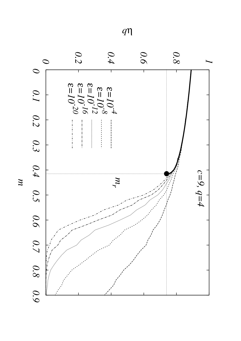
An important simplification of the 1RSB update (20) arises when we consider the soft and the hard fields separately. The fraction of hard fields can be computed using the generalized SP equation (38), provided the ratio is computed. This considerably reduced the size of the population as only soft field has to be kept in memory. Another way to further speed up the code is to generate directly soft fields with a uniform measure instead of waiting for them to come out from the 1RSB recursion. Indeed they might be quite rare in the region of small and one can spend a considerable amount of time before being able to sample them correctly. Generating the soft fields with a uniform weight turns out to be rather easy using the following method: (i) Choose two random colors and . (ii) Perform the usual recursion (31) in order to have a new vector but forbid incoming hard fields to and . (iii) To obtain a uniform soft field generator, the resulting field should be weighted by where is the number of non-null components in the vector. This is specially useful in the case of Erdős-Rényi graphs.
The formula for the free entropy (32) also simplifies in this case. Consider a given site ; the site free entropy term can be split into three parts when (i) the field is hard, (ii) the total field is soft and (iii) the field is contradictory. Then
| (74) |
where / are the probabilities that the total field is frozen/soft, and are given by the SP recursion. Indeed the probability that the total field is not contradictory () is the denominator in eq. (35) while is the numerator of eq. (35). The link part can also be simplified using the fact that contradictions arise when two incoming frozen messages of the same color are chosen, so that
| (75) |
where is simply .
For the formula further simplify as so that
| (76) | |||||
| (77) |
This is precisely what was obtained within the energetic cavity approach in Coloring. The numerical population dynamics implementation with mixed hard/soft strategy is therefore as precise as it could be since we obtain the exact evaluation in the case. This simple computation also demonstrates how one can recover the energetic zero temperature limit from the generic formalism.
Finally, we obtain the function . We fit this function using an ansatz and then perform the Legendre transform to obtain the entropy and complexity. It is also possible to compute directly the complexity from the population data using the expression of the derivative of the potential directly in the code. Both methods lead to very good results. We show an example of the raw data and their fit in fig. 15, where the data have been obtained with relatively small population but where the mixed strategy separating the hard and soft fields have been used. For the purely soft-field branch, we used . It took few hours up to few days to generate these curves on present Intel PCs.


In the case of bi-regular random graphs, one needs two different populations: one for the fields going from nodes with connectivity and one for the fields going from nodes with connectivity . Then each iteration for population (resp. ) should be performed using as incoming messages the vectors of population (resp. 1.). Again, one can separately perform the recursion for the hard-field fractions in both population.
The case of Erdős-Rényi random graphs is more involved, as one needs a large number of populations, each of them of size . In this case, using the separate hard/soft fields implementation and the formulae (74,75) for complexity is crucial, as it allows a good precision even for smaller population sizes. We used typically and . The error bars in table 2 are computed from several independent runs of the population dynamics. In each case we were able to make the equilibration times and the population sizes large enough such that by doubling the time or the population size we did not observed any significant systematic changes in the average results.
Appendix E High- asymptotics
The quenched averages in the large limit are the same for the regular and Erdős-Rényi graphs and we thus consider directly the regular ensemble of connectivity . The appearance of a nontrivial 1RSB solution for , which correspond to , was already computed in ColoringFlo and reads
| (78) | |||||
| (79) |
while the coloring threshold is ColoringFlo
| (80) |
We now show how the connectivity where a solution with hard fields at first appears, and how the complete free entropy (30) can be computed close to the COL/UNCOL transition
E.1 The appearance of hard fields at
We first show that the correct scaling for the appearance of hard fields at is
| (81) |
and compute the value of . In the order we can write also . The starting point is the equation (72), with . In the large limit the fraction of hard fields is , where is the fraction of soft fields. We check self-consistently at the end of the computation that only the two first terms of (72) are important. Then we have
| (82) |
A self-consistent equation for follows
| (83) |
which is solved by where
| (84) |
The maximum of the left hand side is for . It means that a solution of (84) exists for . Finally the hard fields appear in the 1RSB solution for at connectivity
| (85) |
The clustering transition should be between and as this is what we observed for finite . We see that and differs only in the third order and both are very far from the coloring threshold and also from the condensation transition as we show in section E.2. It would be interesting to compute a large expansion of the connectivity at which the hard fields appears in all the clusters (for all such that ). Together with our conjecture about rigidity being responsible for the computational hardness that might give a hint about the answer on the long-standing question FrMcDi: “Is there a polynomial algorithm and such that the algorithm would color random graphs of average connectivity for all large ?”
E.2 The condensation transition
To compute the large- asymptotic of the condensation transition, we first need to derive the large- expansion of the free entropy (30) in the connectivity regime . Let us show self-consistently that the following scaling is relevant for the condensation transition in the large limit
| (86) | |||||
| (87) |
and compute the constants , , . Using the above scaling, the function (35) is dominated by the first two terms in numerator and denominator, and reads in the first two leading orders so that
| (88) |
independently of , , and . To take into account the reweighting we expand eq. (38) in the two leading orders
| (89) |
Note that almost all the incoming fields are hard, i.e. have one component of value . Since there are on average only incoming soft fields, the leading order of the hard-field reweighting (the normalization in eq. (4)) is different from with a probability only . Similarly, almost all the soft fields have two nonzero and equal components. The normalization in eq. (4) is thus almost surely , thus the average reweighting factor of the soft fields is
| (90) |
Finally,
| (91) |
Therefore the constant in (87) is , independently of and .
The computation of the complexity requires the next order in the hard-field reweighting. Indeed the normalization in (4) might not be but ; and this happens when there is a soft field arriving of the color corresponding to the hard field in consideration. The probability of this event is . The hard-field reweighting is thus
| (92) |
We now expand the replicated free energy (30) in the large limit and regime (86). Remind that from (6, 8)
| (93) |
The averages are over the population in the sense of (21).
The site free energy is the logarithm of the average of the total field normalization. This average can be split into three parts when (i) the total field is a hard field, (ii) the total field is a soft field and (iii) the total field is contradictory (and its normalization zero). The probability that the total field is not contradictory is the denominator in eq. (35)
| (94) |
where again only the first two terms are relevant in the expansion. The site free energy is then
| (95) | |||||
where
| (96) | |||||
| (97) |
To compute the link contribution in (93) we need to consider two fields and and to compute
| (98) |
There are three different cases:
- 1.
Two hard fields are chosen, then with probability (this is of order ) and with probability (this is of order ).
- 2.
Two soft fields are chosen then with probability (this is of order ), all other situations being . Let us remind that the dominant soft fields are two-component of type .
- 3.
One hard and one soft field is chosen, then with probability , and with probability (this is of order ).
On average, one thus obtain for the link contribution
| (99) |
Putting together the two pieces (95) and (99), expanding according to (91) and considering only the highest order in , we can finally write the free energy as
| (100) |
The internal entropy and the complexity are then
| (101) | |||||
| (102) |
and the complexity is thus zero for . In particular, one has for the coloring and the condensation thresholds
| (103) | |||||
| (104) |
For connectivity , one gets
| (105) | |||||
| (106) |
References
- (1) S. Cook, Proceedings of the 3rd Annual ACM Symposium. on Theory of Computing (ACM, New York, 1971), pp. 151-158. M. R. Garey and D. S. Johnson Computers and Intractability: A Guide to the Theory of NP-Completeness, (Freeman, New York, 1979). C.H Papadimitrious, Computational complexity (Addison-Wesley, 1994).
- (2) K. Appel and W. Haken, Illinois J. Math. 21, 421 (1977). K. Appel and W. Haken, Illinois J. Math. 21, 491 (1977).
- (3) R. E. Miller and J. W. Thatcher (eds.), Complexity of Computer Computation, Plenum Press. New York, 85 (1972).
- (4) B. Bollobás, Random Graphs (CUP, Cambridge, 2001).
- (5) S.Janson, T. Luczak and A.Rucinski, Random Graphs, John Wiley and Sons, 2000.
- (6) P. Erdős and A. Rényi, Publ. Math. (Debrecen) 6, 290 (1959).
- (7) D. Achlioptas and E. Friedgut, Random Structures and Algorithms, Volume 14, Issue 1, Pages 63 - 70 (1999).
- (8) D. Achlioptas, A. Naor, Y. Peres, Nature, 435 (2005), 759-764.
- (9) S. Dubois, O. Mandler, unpublished.
- (10) D. Achlioptas, C. Moore, Journal of Comp. & Sys. Sci., 67 (2), (2003), p.441-471.
- (11) D. Achlioptas, C. Moore, Proc. RANDOM 2004.
- (12) L. Shi, N.C. Wormald, Research Report CORR 2004-24, Faculty of Mathematics, University of Waterloo (September 2004).
- (13) G. Kemkes, N.C. Wormald, Research Report CORR 2005-22, Faculty of Mathematics, University of Waterloo (2005).
- (14) J. Díaz, G. Grammatikopoulos, A.C. Kaporis, L.M. Kirousis, X. Perez, and D.G. Sotiropoulos; Proceedings of the 13th Annual European Symposium on Algorithms, 2005.
- (15) T. Luczak, Combinatorica 11, 45 (1991).
- (16) P. Cheeseman, B. Kanefsky, W.M. Taylor, Proceedings of the Twelfth International Joint Conference on Artificial Intelligence, IJCAI-91, Sydney, Australia, 1991.
- (17) B. Selman, S. Kirkpatrick, Artificial Intelligence 81 (1-2): 273-295 MAR 1996. B. Selman, D. G. Mitchell, H. J. Levesque, Artificial Intelligence 81 (1-2): 17-29 MAR 1996.
- (18) D.L. Mammen, T. Hogg, J. Artif. Intell. Res. (JAIR) 7: 47-66 (1997).
- (19) C. P. Williams, T. Hogg, Artificial Intelligence 70 (1-2): 73-117 OCT 1994, T. Hogg, B. A. Huberman and C. P. Williams, Artificial Intelligence 81 (1-2): 1-15 MAR 1996.
- (20) S. Cocco and R. Monasson, Phys. Rev. Lett. 86 (8): 1654-1657 FEB 19 2001.
- (21) D. Achlioptas and M. Molloy, in Proc. of FOCS-97 (IEEE, New York, 1997).
- (22) A. Frieze and C.J.H. McDiarmid, Rand. Struc. Alg. 10, 5 (1996).
- (23) R. Monasson, R. Zecchina, S. Kirkpatrick, B. Selman, and L. Troyansky, Nature 400, 133 (1999).
- (24) M. Mézard, Parisi G and Zecchina R, Science 297, 812 (2002).
- (25) F.Y. Wu, Rev. Mod. Phys. 54, 235 (1982).
- (26) Mézard M and Parisi G, 2001 Eur. Phys. J. B 20 217.
- (27) Mézard M and Parisi G, 2003 J. Stat. Phys 111 no. 1-2, 1-34.
- (28) M. Mézard and R. Zecchina, Phys. Rev. E, 66, 056126, (2002).
- (29) Mézard M, Parisi G and Virasoro M A, Spin-glass Theory and Beyond, vol. 9 of Lecture notes in Physics. World Scientific, Singapore, 1987
- (30) R. Mulet, A. Pagnani, M. Weigt and R. Zecchina, Phys. Rev. Lett. 89, 268701 (2002). A. Braunstein, R. Mulet, A. Pagnani, M. Weigt, and R. Zecchina, Phys. Rev. E 68, 036702 (2003).
- (31) F. Krzakala, A. Pagnani, and M. Weigt, Phys. Rev. E 70, 046705 (2004).
- (32) J. van Mourik and D. Saad, Phys. Rev. E 66, 056120 (2002).
- (33) A. Braunstein, M. Mézard, and R. Zecchina, Random Struct. Algorithms 27, 201 (2005).
- (34) Montanari A, Parisi G and Ricci-Tersenghi F, J. Phys. A: Math. Gen. 37 2073-2091.
- (35) G. Biroli, R. Monasson, M. Weigt, Eur. Phys. J. B 14, 551 (2000).
- (36) M. Mézard, T. Mora and R. Zecchina, Phys. Rev. Lett. 94, 197205 (2005).
- (37) D. Achlioptas, F. Ricci-Tersenghi, Proc. 38th annual ACM symposium on Theory of computing (2006), p. 130.
- (38) M. Mézard, M. Palassini and O. Rivoire, Phys. Rev. Lett. 95, 200202 (2005).
- (39) O. Rivoire, These de doctorat, CNRS http://tel.ccsd.cnrs.fr/tel-00009956/en/ (2005).
- (40) Pearl J, Probabilistic Reasoning in Intelligent Systems: Networks of Plausible Inference (2nd edition). Morgan Kaufmann Publishers, San Francisco, 1988.
- (41) Yedidia, J.S., Freeman, W.T. and Weiss, Y., Exploring Artificial Intelligence in the New Millennium, ISBN 1558608117, Chap. 8, pp. 239-236, January 2003 (Science and Technology Books).
- (42) F. Krzakala, A. Montanari, F. Ricci-Tersenghi, G. Semerjian, L. Zdeborová, Proc. Natl. Acad. Sci. 104, 10318 (2007).
- (43) A. Montanari, F. Ricci-Tersenghi, G. Semerjian, in preparation (2007).
- (44) D. J. Gross, I. Kanter and H. Sompolinsky Phys. Rev. Lett. 55, 304-307 (1985).
- (45) H. O. Georgii, Gibbs Measures and Phase Transitions, Berlin (1988).
- (46) S. Franz, M. Mézard, F. Ricci-Tersenghi, M. Weigt and R. Zecchina, Europhys. Lett. 55 (2001) 465.
- (47) H. A. Bethe, Proc. R. Soc. Lond. 150, 552 (1935). R. Peierls, Proc. Roy. Soc. 154, 207 (1936). L Onsager - Journal of the American Chemical Society, (1936). P. R. Weiss, Phys. Rev. 74, 1493 - 1504 (1948).
- (48) K.Y. Wong and D. Sherrington, J. Phys. A 21 (1988) L459. Y.Y. Goldschmidt and P.-Y.Lai, J. Phys.A 23 (1990) L775.
- (49) D. Aldous, The zeta(2) Limit in the Random Assignment Problem. Random Structures and Algorithms 18 (2001) 381-418.
- (50) Bandyopadhyay A and Gamarnik D, 2006 ACM-SIAM Symp. on Discrete Algorithms, 890.
- (51) J. Jonasson, Statistics and Probability Letters 57 (2002), 243-248.
- (52) A. Montanari, Devavrat Shah, Proceedings of Symposium of Discrete Algorithms (SODA), New Orleans, September 2007.
- (53) M. Mézard, A. Montanari, J. Stat. Phys. 124, 1317-1350 (2007).
- (54) J.P. Bouchaud, G. Biroli, J. Chem. Phys. 121, 7347 (2004).
- (55) A. Montanari, G. Semerjian, J. Stat. Phys. 124, 103-189 (2006); Phys. Rev. Lett. 94, 247201 (2005)
- (56) O. Rivoire, G. Biroli, O. C. Martin, M. Mézard, Eur. Phys. J. B 37, 55-78 (2004).
- (57) H. Kesten, B. P. Stigum, Ann Math Statist 37, 1463 (1966). H. Kesten, B. P. Stigum, J Math Anal Appl 17, 309 (1966)
- (58) Parisi G, J. Phys. A13 L115-L121, (1980).
- (59) R. Monasson. Phys. Rev. Lett. 75, 2847 (1995).
- (60) B. Derrida, Phys. Rev. Lett. 45, 79-82 (1980). B. Derrida, Phys. Rev. B 24, 2613-2626 (1981).
- (61) T. Kirkpatrick and D. Thirumalai, Phys. Rev. Lett. 58, 2091 (1987). T. Kirkpatrick, D. Thirumalai, and P. Wolynes, Phys. Rev. A 40, 1045 (1989). M. Mézard and G. Parisi, Phys. Rev. Lett. 82 (1999) 747. M. Mézard, in ”More is different”, Ong and Bhatt editors, Princeton (2002).
- (62) A. Montanari, G. Semerjian, J. Stat. Phys. 125, 23 (2006).
- (63) W Kauzmann, Chemical Reviews 43 (2), 1948.
- (64) G. Semerjian, arXiv:0705.2147v1 (2007).
- (65) G. Parisi, cs.CC/0212047.
- (66) E. N. Maneva, E. Mossel and M. J. Wainwright, in Proceedings of SODA, 2005.
- (67) A. Braunstein, R. Zecchina, J. Stat. Mech. P06007 (2004).
- (68) B. Pittel, J. Spencer, N. Wormald, J. of Combinatorial Theory, Series B, 67, 1996, pp. 111–151.
- (69) E. Gardner, Nucl. Phys. B297, [FS14] 74 (1985).
- (70) A. Montanari and F. Ricci-Tersenghi, Eur. Phys. J. B 33, 339 (2003)
- (71) G. Parisi and T. Rizzo, Phys. Rev. B 72, 184431 (2005). M. Müller, L. Leuzzi, and A. Crisanti, Phys. Rev. B 74, 134431 (2006).
- (72) C.S. O’Hern, L. E. Silbert, A. J. Liu and S. R. Nagel, Phys. Rev. E 68, 011306 (2003).
- (73) F. Krzakala and J. Kurchan, cond-mat/0702546.
- (74) J. Chavas, C. Furtlehner, M. Mézard and R. Zecchina, J. Stat. Mech. (2005) P11016
- (75) P. Svenson, G. Nordahl, Phys. Rev. E, 59, n. 4, 3983 (1999).
- (76) B. Selman, H. A. Kautz and B. Cohen, proc. of AAAI-94, Seattle (1994);
- (77) J. Ardelius, E. Aurell, Phys. Rev. E 74, 037702 (2006).
- (78) S. Seitz, M. Alava, P. Orponen, J Stat. Mech. (2005) P06006.
- (79) S. Boettcher and A. G. Percus, Phys. Rev. E 64,026114(2001).
- (80) Mézard M., Parisi G., Virasoro M.A., J. Physique Lett. 46 (1985) L-217.
- (81) M. Talagrand , Spin Glasses: A challenge for Mathematicians, Springer, 2000.
- (82) Pitman J., Yor M., Ann. Probab. 25, 855-900 (1997).
- (83) L. Devroye, Non-Uniform Random Variate Generation, Springer-Verlag, New York, 1986
- (84) T. Castellani, F. Krzakala and F. Ricci-Tersenghi; Eur. Phys. J. B 47, 99 (2005)