Plasmaneutrino spectrum

A. Odrzywołek Affiliation: M. Smoluchowski Institute of Physics, Jagiellonian University, Reymonta 4, 30-059 Krakow, Poland

August 11, 2026

Abstract

Spectrum of the neutrinos produced in the massive photon and longitudal plasmon decay process has been computed with four levels of approximation for the dispersion relations. Some analytical formulae in limiting cases are derived. Interesting conclusions related to previous calculations of the energy loss in stars are presented. High energy tail of the neutrino spectrum is shown to be proportional to exp(-E/kT), where E is the neutrino energy and kT is the temperature of the plasma.

pacs

97.90.+j and 97.60.-s and 95.55.Vj and 52.27.Ep

1 Introduction & Motivation

Thermal neutrino loses from plasma are very important for stellar astrophysics Arnett; Bisnovaty. Plasmon decay is one of the three main reactions. Extensive calculations for these processes were done by group of Itoh Itoh_I; Itoh_I_erratum; Itoh_II; Itoh_III; Itoh_III_erratum; Itoh_IV; Itoh_V; Itoh_VI; Itoh_VII. Other influential article include BPS; Adams-Woo; Dicus; BraatenSegel; BraatenPRL; Schinder; BlinnikovRudzskij; BlinnikovRudzskij2; Raffelt. Meanwhile, our abilities to detect neutrinos has grown by many orders of magnitude, beginning with $1.4$ tonne experiment of Reines&Cowan ReinesCowan up to the biggest existing now $50$ kt Super-Kamiokande detector SK. Recently, ”GADZOOKS!” upgrade to Super-Kamiokande proposed by Beacom&Vagins Gadzooks attract attention of both experimental and theoretical physicists. At last one new source of the astrophysical antineutrinos is guaranteed with this upgrade, namely Diffuse Supernova Neutrino Background SN1987A-20th; DSNB. Pre-supernova stars will be available to observations out to $\sim$ 2 kiloparsecs SN1987A-20th. This technique is the only extensible to megaton scale SN1987A-20th. Memphys, Hyper-Kamiokande and UNO (Mt-scale water Cherenkov detectors cf. e.g. Fogli) proposals now seriously consider to add GdCl₃ to the one of the tanks with typical three-tank design NNN06. Recently, the discussion on the geoneutrino detection Learned_GEO, increased attention to the deep underwater neutrino observatories HanoHano with target mass 5-10 Mt SN1987A-20th and even bigger GigatonArray. It seems that (anti)neutrino astronomy is on our doorstep, but numerous astrophysical sources of the $\nu$ ’s still are not analyzed from the detection point of view.

Detection of the solar Davis; Gallex; SNO; SK_sun and supernova neutrinos SK_sn; IMB; LSD; Baksan was accompanied and followed with extensive set of detailed calculations (see e.g. Bahcall; MPA; Burrows; Mezzacappa; Yamada; Bethe and references therein as a representatives of this broad subject) of the neutrino spectrum. On the contrary, very little is known about spectral neutrino emission from other astrophysical objects. Usually, some analytical representation of the spectrum is used, based on earlier experience and numerical simulations, cf. e.g. Pons. While this approach is justified for supernovae, where neutrinos are trapped, other astrophysical objects are transparent to neutrinos, and spectrum can be computed with an arbitrary precision. Our goal is to compute neutrino spectra as exact as possible and fill this gap. Plasmaneutrino process dominates dense, degenerate objects like red giant cores RedGiants, cooling white dwarfs WDcool including Ia supernova progenitors before so-called ,,smoldering” phase IaSmouldering. It is also important secondary cooling process in e.g. neutron star crusts HaenselRev and massive stars Heger_rev. Unfortunately, thermal neutrino loses usually are calculated using methods completely erasing almost any information related to the neutrino energy $\mathcal{E}_{\nu}$ and directionality as well. This information is not required to compute total energy $Q$ radiated as neutrinos per unit volume and time. From experimental point of view, however, it is extremely important if given amount of energy is radiated as e.g. numerous keV neutrinos or one 10 MeV neutrino. In the first case we are unable to detect (using available techniques) any transient neutrino source regardless of the total luminosity and proximity of the object. In the second case we can detect astrophysical neutrino sources if they are strong and not too far away using advanced detector which is big enough.

Few of the research articles in this area attempt to estimate average neutrino energy BraatenPRL; Schinder; Ratkovic; Dutta computing additionally reaction rate $R$ . Strangely, they presented figures and formulae for $Q/R$ instead of $\frac{1}{2}Q/R$ . This gives false picture of real situation, as former expression gives $\langle\mathcal{E}_{\nu}+\mathcal{E}_{\bar{\nu}}\rangle$ . Obviously, we detect neutrinos not $\nu$ - $\bar{\nu}$ pairs. $\frac{1}{2}Q/R$ do not give average neutrino energy, as in general neutrino and antineutrino spectra are different. As we will see only for longitudal plasmon decay neutrinos energies of neutrinos and antineutrinos are equal. However, difference in all situations where thermal neutrino loses are important is numerically small and formula:

\langle\mathcal{E}_{\nu}\rangle\simeq\frac{1}{2}\frac{Q}{R}

(1)

is still a ”working” estimate.

Mean neutrino energy is useful in the purpose of qualitative discussion of the detection prospects/methods. Quantitative discussion require knowledge of spectrum shape (differential emissivity $dR/d\mathcal{E}_{\nu}$ ). High energy tail is particularly important from an experimental detection point of view. Detection of the lowest energy neutrinos is extremely challenging due to numerous background signal noise sources e.g. ¹⁴C decay for $\mathcal{E}_{\nu}<200$ keV 14C. Relevant calculations for the spectrum of the medium energy $\langle\mathcal{E}_{\nu}\rangle\sim 1$ MeV neutrinos emitted from thermal processes has become available recently Ratkovic; Dutta; MOK. Purpose of this article is to develop accurate methods and discuss various theoretical and practical (important for detection) aspects of the neutrino spectra from astrophysical plasma process. This could help experimental physicists to discuss possible realistic approach to detect astrophysical sources of the neutrinos in the future.

2 Plasmaneutrino spectrum

2.1 Properties of plasmons

Emissivity and the spectrum shape from the plasmon decay is strongly affected by the dispersion relation for transverse plasmons (massive in-medium photons) and longitudal plasmons. In contrast to transverse plasmons, with vacuum dispersion relation $\omega(k)=k$ , longitudal plasmons exist only in the plasma. Dispersion relation, by the definition is a function $\omega(k)$ where $\hbar\omega$ is the energy of the (quasi)particle and $\hbar k$ is the momentum. Issues related to particular handling of these functions are discussed clearly in the article of Braaten and Segel BraatenSegel. We will repeat here the most important features of the plasmons.

For both types, plasmon energy for momentum $k=0$ is equal to $\omega_{0}$ . Value $\omega_{0}\equiv\omega(0)$ is refereed to as plasma frequency and can be computed from:

\omega_{0}^{2}=\frac{4\alpha}{\pi}\int_{0}^{\infty}\frac{p^{2}}{E}\left(1-\frac{v^{2}}{3}\right)(f_{1}+f_{2})\;dp

(2)

where $v=p/E$ , $E=\sqrt{p^{2}+m_{e}^{2}}$ ( $\hbar=c=1$ units are used), $m_{e}\simeq 0.511$ MeV and fine structure constant is $\alpha=1/137.036$ PDBook. Functions $f_{1}$ and $f_{2}$ are the Fermi-Dirac distributions for electrons and positrons, respectively:

f_{1}=\frac{1}{e^{(E-\mu)/kT}+1},\qquad f_{2}=\frac{1}{e^{(E+\mu)/kT}+1}.

(3)

Quantity $\mu$ is the electron chemical potential (including the rest mass). Other important parameters include first relativistic correction $\omega_{1}$ :

\omega_{1}^{2}=\frac{4\alpha}{\pi}\int_{0}^{\infty}\frac{p^{2}}{E}\left(\frac{5}{3}v^{2}-v^{4}\right)(f_{1}+f_{2})\;dp

(4)

maximum longitudal plasmon momentum (energy) $k_{max}$ :

k_{max}^{2}\equiv\omega_{max}^{2}=\frac{4\alpha}{\pi}\int_{0}^{\infty}\frac{p^{2}}{E}\left(\frac{1}{v}\ln{\frac{1-v}{1+v}}-1\right)(f_{1}+f_{2})\;dp

(5)

and asymptotic transverse plasmon mass $m_{t}$ :

m_{t}^{2}=\frac{4\alpha}{\pi}\int_{0}^{\infty}\frac{p^{2}}{E}(f_{1}+f_{2})\;dp.

(6)

Value $m_{t}$ is often referred to as thermal photon mass. We also define parameter $v_{\ast}$ :

v_{\ast}=\frac{\omega_{1}}{\omega_{0}}

(7)

interpreted as typical velocity of the electrons in the plasma BraatenSegel. Axial polarization coefficient is:

\omega_{A}=\frac{2\alpha}{\pi}\int_{0}^{\infty}\frac{p^{2}}{E^{2}}\left(1-\frac{2}{3}\,v^{2}\right)(f_{1}-f_{2})\;dp.

(8)

Value of the $\omega_{A}$ is a measure of the difference between neutrino and antineutrino spectra. Set of numerical values used to display sample result is presented in Table 1.

Table 1: Plasma properties for typical massive star during Si burning. All values in MeV.

$kT$	$\mu$	$\omega_{0}$	$\omega_{1}$	$m_{t}$	$\omega_{max}$	$\omega_{A}$
0.32	1.33	0.074	0.070	0.086	0.133	0.002

Values $\omega_{0},\omega_{max},m_{t}$ define sub-area of the $\omega$ - $k$ plane where dispersion relations for photons $\omega_{t}(k)$ and longitudal plasmons $\omega_{l}(k)$ are found:

	$\max{(k,\omega_{0})}\leq\omega_{l}(k)\leq\omega_{max},\quad 0\leq k\leq k_{max}$		(9a)
	$\sqrt{k^{2}+\omega_{0}^{2}}\leq\omega_{t}(k)\leq\sqrt{k^{2}+m_{t}^{2}},\quad\quad 0\leq k\leq\infty$		(9b)

Refer to caption — Figure 1: Longitudal and transverse plasmon dispersion relation $\omega_{l,t}(k)$ for plasma parameters from Table 1. Exact result (dot-sahed) is very close to the Braaten & Segel approximation (solid). Zero-order (dotted) and first order (dashed) approximations are very poor, especially for londitudal mode (left).

Dispersion relations are solution to the equations BraatenSegel:

	$k^{2}=\Pi_{l}\left(\omega_{l}(k),k\right)$		(10a)
	$k^{2}=\omega_{t}(k)^{2}-\Pi_{t}\left(\omega_{t}(k),k\right)$		(10b)

where longitudal and transverse polarization functions are given as an integrals:

	$\Pi_{l}=\frac{4\alpha}{\pi}\int_{0}^{\infty}\frac{p^{2}}{E}\left(\frac{\omega_{l}}{vk}\ln{\frac{\omega_{l}+vk}{\omega_{l}-vk}}\!-\!1-\frac{\omega_{l}^{2}-k^{2}}{\omega_{l}^{2}-v^{2}k^{2}}\right)(f_{1}+f_{2})\;dp.$		(11a)
	$\Pi_{t}=\frac{4\alpha}{\pi}\int_{0}^{\infty}\frac{p^{2}}{E}\left(\frac{\omega_{t}^{2}}{k^{2}}-\frac{\omega_{t}^{2}-k^{2}}{k^{2}}\frac{\omega_{t}}{2vk}\ln{\frac{\omega_{t}+vk}{\omega_{t}-vk}}\right)(f_{1}+f_{2})\;dp.$		(11b)

Typical example of the exact plasmon dispersion relations (dash-dotted) is presented in Fig. 1. As solving eqns. (10a, 10b) with (11) is computationally intensive, three levels of approximation for dispersion relations are widely used:

1.

zero-order analytical approximations
2.

first order relativistic corrections
3.

Braaten&Segel approximation

2.1.1 Approximations for longitudal plasmons

For longitudal plasmons, the simplest zero-order approach used in early calculations of Adams et al. Adams-Woo and more recently in Dutta for photoneutrino process is to put simply:

\omega(k)=\omega_{0}

(12)

where $\omega_{0}$ is the plasma frequency (2). Maximum plasmon energy $\omega_{max}=\omega_{0}$ in this approximation. Zero-order approximation is valid only for non-relativistic regime, and leads to large errors of the total emissivity BPS.

First relativistic correction to (12) has been introduced by Beaudet et al. BPS. Dispersion relation $\omega_{l}(k)$ is given in an implicit form:

\omega_{l}^{2}=\omega_{0}^{2}+\frac{3}{5}\omega_{1}^{2}\frac{k^{2}}{\omega_{l}^{2}},

(13)

with maximum plasmon energy equal to:

\omega_{max}^{(1)}=\sqrt{\omega_{0}^{2}+\frac{3}{5}\omega_{1}^{2}}

(14)

This approximation, however, do not introduce really serious improvement (Figs. 1, 2 (left) & 4). Breaking point was publication of the Braaten&Segel approximation BraatenSegel. Using simple analytical equation:

k^{2}=3\,\frac{\omega_{0}^{2}}{v_{\ast}^{2}}\left(\frac{\omega_{l}}{2v_{\ast}k}\ln{\frac{\omega_{l}+v_{\ast}k}{\omega_{l}-v_{\ast}k}}-1\right)

(15)

where $v_{\ast}$ is defined in (7) one is able to get almost exact dispersion relation, cf. Figs. 1 & 2, left panels. Solution to the eq. (15) exist in the range $1<k<k_{max}^{BS}$ , where, in this approximation, maximum longitudal plasmon momentum is:

\left(\omega_{max}^{BS}\right)^{2}=\frac{3\omega_{0}^{2}}{2v_{\ast}^{2}}\left(\frac{1}{2v_{\ast}}\ln{\frac{1+v_{\ast}}{1-v_{\ast}}}-1\right)

(16)

what gives value slightly different than exact value (Fig. 2, left), but required for consistency of the approximation.

2.1.2 Approximations for transverse plasmons

For photons in vacuum dispersion relation is $\omega_{t}=k$ . Zero order approximation for in-medium photons is:

	$\omega_{t}^{2}=\omega_{0}^{2}+k^{2},\quad k\ll\omega_{0}$	(17a)
valid for small $k$ and:
	$\omega_{t}^{2}=m_{t}^{2}+k^{2},\quad k\gg\omega_{0}$	(17b)

valid for very large $k$ . Formulae (17a) and (17b) provide lower and upper limit for realistic $\omega_{t}(k)$ , respectively (cf. Fig. 1, right panel, dotted). First order relativistic corrections lead to the formula:

\omega_{t}^{2}=\omega_{0}^{2}+k^{2}+\frac{1}{5}\omega_{1}^{2}\frac{k^{2}}{\omega_{t}^{2}}

(18)

with asymptotic photon mass:

m_{t}^{(1)}=\sqrt{\omega_{0}^{2}+\omega_{1}^{2}/5}

(19)

Finally, Braaten&Segel approximation leads to:

\omega_{t}^{2}=k^{2}+\omega_{0}^{2}\frac{3\,\omega_{t}^{2}}{2\,v_{\ast}^{2}\,k^{2}}\left(1-\frac{\omega_{t}^{2}-v_{\ast}^{2}k^{2}}{2\,\omega_{t}\,v_{\ast}\,k}\ln{\frac{\omega_{t}+v_{\ast}k}{\omega_{t}-v_{\ast}k}}\right)

(20)

Asymptotic photon mass $m_{t}^{BS}$ derived from (20) is:

\left(m_{t}^{BS}\right)^{2}=\frac{3\,\omega_{0}^{2}}{2v_{\ast}^{2}}\left(1-\frac{1-v_{\ast}^{2}}{2v_{\ast}}\ln{\frac{1+v_{\ast}}{1-v_{\ast}}}\right)

(21)

This is slightly smaller (left panel of Fig. 2, dashed) than exact value (solid line).

All four relations are presented in Fig. 1. Differences are clearly visible, but they are much less pronounced for transverse than for longitudal plasmons. Inspection of Fig. 2 reveals however, that in the large momentum regime asymptotic behavior is correct only for exact integral relations (10b) and may be easily reproduced using (17b) with $m_{t}$ from (6).

Let us recapitulate main conclusions. Braaten&Segel approximation provide reasonable approximation, as nonlinear equations (15) and (20) are easily solved using e.g. bisection method. Zero and first-order approximations (12, 17a, 17b) with limiting values (9) provide starting points and ranges. Approximation has been tested by Itoh_VIII and is considered as the best available Raffelt. Errors for part of the $kT$ - $\mu$ plane where plasmaneutrino process is not dominant may be as large as 5% Itoh_VIII. At present, these inaccuracies are irrelevant for any practical application, and Braaten&Segel approximation is recommended for all purposes.

2.2 Plasmon decay rate

In the Standard Model of electroweak interactions, massive in-medium photons and longitudal plasmons may decay into neutrino-antineutrino pairs:

\gamma^{\ast}\rightarrow\nu_{x}+\bar{\nu}_{x}.

(22)

In the first-order calculations two Feynmann diagrams (Fig. 3) contribute to decay rate BraatenSegel; Ratkovic.

For the decay of the longitudal plasmon squared matrix element is:

	$M_{l}^{2}=\frac{G_{F}^{2}C_{V}^{2}}{\pi\alpha}\left(\omega_{l}^{2}-k^{2}\right)^{2}\;\Biggl[\frac{2K\cdot Q_{1}\;K\cdot Q_{2}}{K^{2}}+\\ \frac{2\,\mathbf{k}\cdot\mathbf{q}_{1}\;\mathbf{k}\cdot\mathbf{q}_{2}}{k^{2}}-Q_{1}\cdot Q_{2}\Biggr]$		(23a)
where $K=(\omega,\mathbf{k})$ is four momentum of the plasmon. $Q_{1}=(\mathcal{E}_{1},\mathbf{q}_{1})$ and $Q_{2}=(\mathcal{E}_{2},\mathbf{q}_{2})$ is four-momentum of the neutrino and antineutrino, respectively.

Squared matrix element for decay of the massive photon is:

M_{t}^{2}=\frac{G_{F}^{2}}{\pi\alpha}\Biggl[\left(C_{V}^{2}\Pi_{t}^{2}+C_{A}^{2}\Pi_{A}^{2}\right)\left(\mathcal{E}_{1}\mathcal{E}_{2}-\frac{\mathbf{k}\cdot\mathbf{q}_{1}\;\mathbf{k}\cdot\mathbf{q}_{2}}{k^{2}}\right)\\ +2C_{V}C_{A}\Pi_{t}\Pi_{A}\frac{\mathcal{E}_{1}\;\mathbf{k}\cdot\mathbf{q}_{2}-\mathcal{E}_{2}\;\mathbf{k}\cdot\mathbf{q}_{1}}{k}\Biggr]

(23b)

where $\Pi_{t}$ is defined in (11b) and axial polarization function $\Pi_{A}$ reads:

\Pi_{A}=\frac{2\alpha}{\pi}\frac{\omega_{t}^{2}\!-\!k^{2}}{k}\int_{0}^{\infty}\frac{p^{2}}{E^{2}}\left(\frac{\omega_{t}}{2vk}\ln{\frac{\omega_{t}+vk}{\omega_{t}-vk}}\!-\!\frac{\omega_{t}^{2}-k^{2}}{\omega_{t}^{2}-v^{2}k^{2}}\right)(f_{1}-f_{2})\;dp

(24)

Fermi constant is $G_{F}/(\hbar c)^{3}=1.16637(1)\times 10^{-5}\,\mathrm{GeV}^{-2}$ PDBook and, in standard model of electroweak interactions, vector and axial coupling constants are:

C_{V}^{e}=\frac{1}{2}+2\sin^{2}{\theta_{W}},\quad C_{A}^{e}=\frac{1}{2}

(25)

C_{V}^{\mu,\tau}=-\frac{1}{2}+2\sin^{2}{\theta_{W}},\quad C_{A}^{\mu,\tau}=-\frac{1}{2}

(26)

for electron and $\mu,\tau$ neutrinos, respectively. The Weinberg angle is $\sin^{2}{\theta_{W}}=0.23122(15)$ PDBook.

Terms containing $C_{A}$ (so-called axial contribution) in (23b) are frequently treated separately Ratkovic or removed at all Itoh_I. In calculations concentrated on the total emissivity this is justified as anti-symmetric term multiplied by $C_{V}C_{A}$ do not contribute at all and term $C_{A}^{2}\times\ldots$ is suppressed relative to the term beginning with $C_{V}^{2}\times\ldots$ by four orders of magnitude Itoh_I. However, if one attempts to compute neutrino energy spectrum all three terms should be added together, as mixed V-A ,,channel” alone leads to negative emission probability for some neutrino energy range (Fig. 6), what is physically unacceptable. These terms remains numerically small but only for electron neutrinos. For $\mu$ and $\tau$ neutrino spectra axial part contributes at $\sim$ 1% level due to very small value $C_{V}^{\mu,\tau}=-0.0376$ while still $C_{A}=-0.5$ . ”Mixed” term leads to significant differences between $\nu_{\mu,\tau}$ and $\bar{\nu}_{\mu,\tau}$ spectra, cf. Fig. 6. Relative contributions of the three transverse ”channels” for electron and $\mu,\tau$ are presented in Table 2.

Table 2: Relative weight of the

M_{t}^{2}

(23b) terms for

e

and

\mu,\tau

neutrinos.

Flavor	Vector	Axial	Mixed
	$\frac{C_{V}^{2}\omega_{0}^{4}}{(C_{V}\omega_{0}^{2}+C_{A}\omega_{A})^{2}}$	$\frac{C_{A}^{2}\omega_{A}^{2}}{(C_{V}\omega_{0}^{2}+C_{A}\omega_{A})^{2}}$	$\quad\frac{2C_{V}C_{A}\omega_{0}^{2}\omega_{A}}{(C_{V}\omega_{0}^{2}+C_{A}\omega_{A})^{2}}$
electron	0.74	0.02	0.24
mu/tau	0.07	0.39	0.54

In general, all the terms in the squared matrix element (23b) should be added. We have only two different spectra: longitudal and transverse one.

Particle production rate from plasma in thermal equilibrium is:

R_{i}=\frac{g_{i}}{(2\pi)^{5}}\int\;Z_{i}\;f_{\gamma^{\ast}}\;\delta^{4}(K-Q_{1}-Q_{2})\;M_{i}^{2}\,\frac{d^{3}\mathbf{k}}{2\omega_{i}}\,\frac{d^{3}\mathbf{q}_{1}}{2\mathcal{E}_{1}}\,\frac{d^{3}\mathbf{q}_{2}}{2\mathcal{E}_{2}}

(27)

where $i=l$ for longitudal mode and $i=t$ for transverse mode. Bose-Einstein distribution for plasmons $f_{\gamma^{\ast}}$ is:

f_{\gamma^{\ast}}=\frac{1}{e^{\omega_{t,l}/kT}-1}.

(28)

and residue factors $Z_{t,l}$ are expressed by polarization functions $\Pi_{t,l}$ (11b, 11a):

Z_{t}^{-1}=1-\frac{\partial\Pi_{t}}{\partial\omega^{2}}

(29)

Z_{l}^{-1}=-\frac{\omega_{l}^{2}}{k^{2}}\;\frac{\partial\Pi_{l}}{\omega^{2}}.

(30)

For massive photons $g_{t}=2$ and for longitudal plasmon $g_{l}=1$ .

Differential rates¹¹ 1 Double differential rate $d^{2}R_{i}/d\mathcal{E}d\cos{\theta}$ has an identical form as (31) but now four momenta cannot be given explicitly, unless simple analytical approximation for $\omega_{i}(k)$ is used. Analytical approximations for the specrum shape are derived this way. has been derived for the first time in Ratkovic. Here, we present result in the form valid for both types of plasmons, ready for calculations using any available form of dispersion relation:

\frac{d^{2}R_{i}}{d\mathcal{E}_{1}\,d\mathcal{E}_{2}}=\frac{g_{i}}{\pi^{4}}\,Z_{i}M_{i}^{2}f_{\gamma^{\ast}}\,J_{i}\;\mathcal{S}

(31)

where $i=l$ or $i=t$ . Product $\mathcal{S}$ of the unit step functions $\Theta$ in (31) restrict result to the kinematically allowed area:

\mathcal{S}=\Theta(4\mathcal{E}_{1}\mathcal{E}_{2}-m_{i}^{2})\Theta(\mathcal{E}_{1}+\mathcal{E}_{2}-\omega_{0})\Theta(\omega_{max}-\mathcal{E}_{1}-\mathcal{E}_{2})

(32)

Four-momenta in the squared matrix element are:

$\displaystyle Q_{1}$	$\displaystyle=$	$\displaystyle(\mathcal{E}_{1},0,0,\mathcal{E}_{1})$
$\displaystyle Q_{1}$	$\displaystyle=$	$\displaystyle(\mathcal{E}_{2},\mathcal{E}_{2}\sin{\theta},0,\mathcal{E}_{2}\cos{\theta})$
$\displaystyle K$	$\displaystyle=$	$\displaystyle(\mathcal{E}_{1}+\mathcal{E}_{2},\mathcal{E}_{2}\sin{\theta},0,\mathcal{E}_{1}+\mathcal{E}_{2}\cos{\theta})$
$\displaystyle m_{i}^{2}$	$\displaystyle=$	$\displaystyle K\cdot K=(\mathcal{E}_{1}+\mathcal{E}_{2})^{2}-k^{\prime 2}$
$\displaystyle\cos{\theta}$	$\displaystyle=$	$\displaystyle\frac{{k^{\prime}}^{2}-\mathcal{E}_{1}^{2}-\mathcal{E}_{2}^{2}}{2\mathcal{E}_{1}\mathcal{E}_{2}}$
$\displaystyle k^{\prime}$	$\displaystyle=$	$\displaystyle\omega_{l,t}^{-1}(\mathcal{E}_{1}+\mathcal{E}_{2})$
$\displaystyle\omega_{i}$	$\displaystyle=$	$\displaystyle\mathcal{E}_{1}+\mathcal{E}_{2}$

where $\omega_{i}^{-1}$ denotes function inverse to the dispersion relation. Jacobian $J_{i}$ arising from Dirac delta integration in (27) is:

J_{i}^{-1}=\frac{\mathcal{E}_{1}\mathcal{E}_{2}}{k^{\prime}}\frac{\partial\omega_{i}}{\partial k}\Bigg|_{k=k^{\prime}}.

(33)

Residue factors $Z_{i}$ are given in (30) and (29). Maximum energy $\omega_{max}$ in (32) for longitudal plasmons must be in the agreement with particular approximation used for $\omega_{l}(k)$ : $\omega_{0}$ , (14) or (16) for zero-order (12), first-order (13) or Braaten&Segel (15) approximation, respectively. For transverse plasmons $\omega_{max}\to\infty$ and last $\Theta$ function in (32) has no effect and may be omitted.

2.3 Longitudal neutrino spectrum

2.3.1 Analytical approximation

We begin with general remark on the spectrum. Note, that eq. (31) is symmetric for longitudal mode under change $\mathcal{E}_{1,2}\to\mathcal{E}_{2,1}$ because (23a) is symmetric with respect to exchange $Q_{1,2}\to Q_{2,1}$ . Resulting energy spectrum is thus identical for neutrinos and antineutrinos. This is not true for transverse plasmons with axial contribution included, cf. Sect. 2.4.

Using zero-order dispersion relation for longitudal plasmons (12) we are able to express spectrum by the elementary functions. Longitudal residue factor $Z_{t}$ is now:

Z_{l}^{0}=1,

(34)

and Jacobian $J_{l}$ resulting from the integration of the Dirac delta function is:

J_{l}^{0}=1.

(35)

Now, differential rate $d^{2}R/d\mathcal{E}d\cos{\theta}$ (cf. (31) and footnote 1) becomes much more simple and integral over $d\cos{\theta}$ can be evaluated analytically. Finally, we get the longitudal spectrum:

\frac{dR}{d\mathcal{E}}\equiv\lambda(\mathcal{E})=\frac{{G_{F}}^{2}\,{C_{V}}^{2}\,{\omega_{0}}^{7}}{1260\,\pi^{4}\,\alpha\,\hbar^{3}\,c^{9}}\;\frac{f(\mathcal{E}/\omega_{0})}{e^{\omega_{0}/kT}-1}

(36)

where normalized spectrum is:

	$\displaystyle f(x)$	$\displaystyle=$	$\displaystyle\frac{105}{32}\;\Bigl[4x(x-1)(8x^{4}-16x^{3}+2x^{2}+6x-3)$		(37)
		$\displaystyle+$	$\displaystyle 3(1-2x)^{2}\ln(1-2x)^{2}\Bigr]$		(37)

Let us note that $f$ is undefined at $x=1/2$ ; use limit instead:

\lim_{x\to 1/2}f(x)=105/32.

Function $f(x)$ is symmetric with respect to point $x=1/2$ , where $f$ has a maximum value (Fig. 4, dotted line).

In this limit, correct for non-relativistic, non-degenerate plasma, average neutrino and antineutrino energy is $\langle\mathcal{E}\rangle=\omega_{0}/2$ and maximum $\nu$ energy is $\omega_{0}$ .

Inspection of Fig. 4 reveals little difference between analytical result (36) and result obtained with first-order relativistic corrections to the dispersion relation (13).

2.3.2 Numerical results

Simple formula (36) significantly underestimates flux and the maximum neutrino energy, equal to $\omega_{max}$ rather than $\omega_{0}$ . Therefore we have used Braaten & Segel approximation for longitudal plasmon dispersion relation.

To derive spectrum we will use form of differential rate (31) provided by Ratkovic. In the Braaten&Segel approximation:

Z_{l}^{BS}=\frac{\omega_{l}^{2}}{\omega_{l}^{2}-k^{2}}\;\frac{2(\omega_{l}^{2}-v_{\ast}^{2}k^{2})}{3\omega_{0}^{2}-\omega_{l}^{2}+v_{\ast}^{2}k^{2}},

J_{l}^{BS}=\left|\frac{k^{2}}{\mathcal{E}_{1}\mathcal{E}_{2}}\frac{1-\beta_{l}}{\omega_{l}\beta_{l}}\right|,

\beta_{l}^{BS}=\frac{3\omega_{0}^{2}}{2v_{\ast}^{3}}\left(\frac{3\omega_{l}}{2k^{3}}\ln{\frac{\omega_{l}+v_{\ast}k}{\omega_{l}-v_{\ast}k}}-\frac{\omega_{l}^{2}v_{\ast}}{k^{2}(\omega_{l}^{2}-v_{\ast}^{2}k^{2})}-\frac{2v_{\ast}}{k^{2}}\right).

Spectrum is computed as an integral of (31) over $d\mathcal{E}_{2}$ . Example result is presented in Fig. 4. Integration of the function in Fig. 4 over neutrino energy gives result in well agreement with both (30) from BraatenSegel and (54) from Ratkovic.

2.4 Transverse plasmon decay spectrum

2.4.1 Analytical approximation

Derivation of massive in-medium photon decay spectrum closely follows previous subsection. Semi-analytical formula can be derived for dispersion relations (17). For dispersion relation (17b) transverse residue factor $Z_{t}$ is:

Z_{t}^{0}=1,

(38)

polarization function $\Pi_{t}$ is equal to:

\Pi_{t}^{0}=m_{t}^{2},

(39)

and Jacobian resulting from integration of the Dirac delta function $J_{t}$ is:

J_{t}^{0}=\frac{\mathcal{E}_{1}+\mathcal{E}_{2}}{\mathcal{E}_{1}\mathcal{E}_{2}}.

(40)

Approximate spectrum, neglecting differences between neutrinos and antineutrinos, is given by the following integral:

\lambda(\mathcal{E})=\frac{G_{F}^{2}C_{V}^{2}}{64\,\pi^{4}\alpha}\frac{m_{t}^{7}}{\hbar^{3}c^{9}}\int_{-1}^{1}\frac{P(\cos{\theta},\mathcal{E}/m_{t})\;d\cos{\theta}}{\exp\left[(\mathcal{E}+\frac{m_{t}^{2}}{2\mathcal{E}(1-\cos{\theta})})/kT\right]-1}

(41)

where rational function $P(ct,x)$ is:

P=\frac{1+2(ct-1)^{2}(2x^{2}-1)x^{2}}{x(ct-1)^{2}[1-2ct(ct-1)x^{2}+2(ct-1)^{2})x^{4}]}

(42)

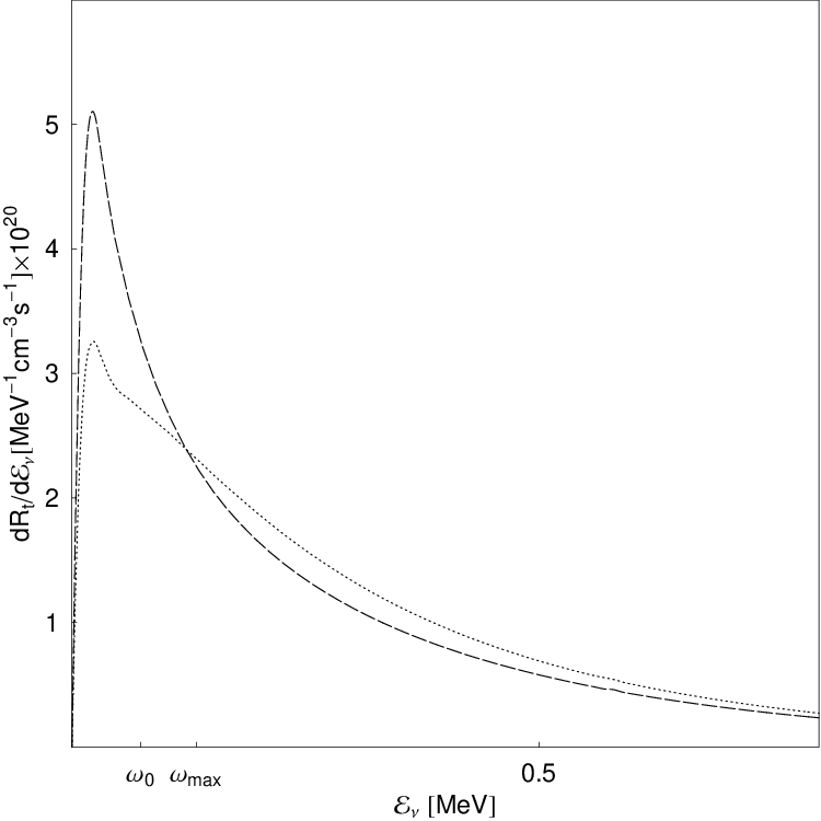
Result presented in Fig. 5 show that spectrum (41) obtained with dispersion relation (17b) agree well in both low and high neutrino energy part with spectrum obtained from Braaten&Segel approximation for dispersion relations. Dispersion relation (17a) produces much larger error, and spectrum nowhere agree with correct result. This fact is not a big surprise: as was pointed out by Braaten BraatenPRL dispersion relation is crucial. Therefore, all previous results, including seminal BPS work BPS, could be easily improved just by the trivial replacement $\omega_{0}\to m_{t}$ . Moreover, closely related photoneutrino process also has been computed BPS; Itoh_I; Schinder; Dicus with simplified dispersion relation (17a) with $\omega_{0}$ . One exception is work of Esposito et. al. Esposito. It remains unclear however, which result is better, as accurate dispersion relations have never been used within photoneutrino process context. For plasmaneutrino, Eq. (17b) is much better approximation than (17a), especially if one put $m_{t}$ from exact formula (6). High energy tail of the spectrum also will be exact in this case.

As formula (41) agree perfectly with the tail of the spectrum, we may use it to derive very useful analytical expression. Leaving only leading terms of the rational function (42)

P(ct,x)\sim x^{-1}(1-ct)^{-2}

one is able to compute integral (41) analytically:

\lambda(\mathcal{E})\simeq\frac{G_{F}^{2}C_{V}^{2}}{64\,\pi^{4}\alpha}\frac{m_{t}^{6}}{\hbar^{3}c^{9}}\left[\kappa-\frac{2}{a}\ln{\left(e^{a\kappa/2}-1\right)}\right]

(43)

where $\kappa=2x+(2x)^{-1}$ , $x=\mathcal{E}/m_{t}$ , $a=m_{t}/kT$ . Interestingly, spectrum (43) is invariant under transformation:

\mathcal{E}^{\prime}\mathcal{E}=m_{t}^{2}/4

and all results obtained for high energy tail of the spectrum immediately may be transformed for low-energy approximation. The asymptotic behavior of (43) for $\mathcal{E}\gg kT$ is of main interest:

\lambda(\mathcal{E}_{\nu})=A\;kT\,m_{t}^{6}\,\exp{\left(-\frac{\mathcal{E}_{\nu}}{kT}\right)}

(44)

where for electron neutrinos :

A=\frac{G_{F}^{2}C_{V}^{2}}{8\pi^{4}\alpha}\frac{1}{\hbar^{4}c^{9}}=2.115\times 10^{30}\;[\mathrm{MeV}^{-8}\mathrm{cm}^{-3}\mathrm{s}^{-1}]

and $m_{t}$ , $kT$ are in MeV. For $\mu,\tau$ neutrinos just replace $A$ with $A\,(C_{V}^{\mu,\tau}/C_{V}^{e})^{2}$ .

Formula (44) gives also quite reasonable estimates of the total emissivity $Q_{t}$ and mean neutrino energies $\langle\mathcal{E}_{\nu}\rangle$ :

	$Q_{t}=A\;kT^{3}\,m_{t}^{6}$		(45a)
	$\langle\mathcal{E}_{\nu}\rangle=kT$		(45b)

For a comparison, Braaten & Segel BraatenSegel derived exact formulae in the high temperature limit $kT\gg\omega_{0}$ :

	$Q_{t}^{BS}=\frac{G_{F}^{2}C_{V}^{2}\zeta(3)}{12\pi^{4}\alpha}\;kT^{3}\,m_{t}^{6}=0.8\,A\;kT^{3}\,m_{t}^{6}$		(46a)
	$\langle\mathcal{E}_{\nu}^{BS}\rangle=\frac{6\zeta(3)}{\pi^{2}}kT=0.73\,kT$		(46b)

Formulae above agree with $\sim$ 25% error in the leading coefficients.

2.4.2 Numerical results

Calculation of the spectrum in the framework of Braaten&Segel approximation requires residue factor, polarization function BraatenSegel (transverse&axial) and Jacobian Ratkovic:

Z_{t}^{BS}=\frac{2\,\omega_{t}^{2}\,(\omega_{t}^{2}-v_{\ast}^{2}\,k^{2})}{3\,\omega_{0}^{2}\omega_{t}^{2}+(\omega_{t}^{2}+k^{2})(\omega_{t}^{2}-v_{\ast}^{2}\,k^{2})-2\,\omega_{t}^{2}(\omega_{t}^{2}-k^{2})},

(47)

\Pi_{t}^{BS}=\frac{3\,\omega_{0}^{2}}{2v_{\ast}^{2}}\left(\frac{\omega_{t}^{2}}{k^{2}}-\frac{\omega_{t}^{2}-v_{\ast}^{2}k^{2}}{k^{2}}\,\frac{\omega_{t}}{2v_{\ast}k}\ln{\frac{\omega_{t}+v_{\ast}k}{\omega_{t}-v_{\ast}k}}\right),

(48)

\Pi_{A}^{BS}=\omega_{A}\,k\;\frac{\omega_{t}^{2}-k^{2}}{\omega_{t}^{2}-v_{\ast}^{2}k^{2}}\;\frac{3\,\omega_{0}^{2}-2\,(\omega_{t}^{2}-k^{2})}{\omega_{0}^{2}},

(49)

J_{t}^{BS}=\frac{\mathcal{E}_{1}+\mathcal{E}_{2}}{\mathcal{E}_{1}\mathcal{E}_{2}}\left|\frac{1-\beta_{t}^{BS}}{1-\frac{\omega_{t}^{2}}{k^{2}}\beta_{t}^{BS}}\right|

(50)

\beta_{t}^{BS}=\frac{9\omega_{0}^{2}}{4v_{\ast}^{2}k^{2}}\left[1+\frac{1}{6}\left(\frac{v_{\ast}k}{\omega_{t}}-\frac{3\omega_{t}}{v_{\ast}k}\right)\ln{\frac{\omega_{t}+v_{\ast}k}{\omega_{t}-v_{\ast}k}}\right]

(51)

Example spectrum, computed as an integral of (31) over $d\mathcal{E}_{2}$ is shown in Fig. 5.

3 Summary

Main new results presented in the article are analytical formulae for neutrino spectra (36, 41) and exact analytical formula (44) for the high energy tail of the transverse spectrum. The latter is of main interest from the detection of astrophysical sources point of view: recently available detection techniques are unable to detect keV plasmaneutrinos emitted with typical energies $\langle\mathcal{E}_{\nu}\rangle\sim\omega_{0}/2$ (Fig. 4, 5), where $\omega_{0}$ is the plasma frequency (2). Tail behavior of the transverse spectrum quickly ”decouple” from $\omega_{0}$ dominated maximum area, and becomes dominated by temperature-dependent term $\exp{(-\mathcal{E}_{\nu}/kT)}$ . Calculation of the events in the detector is then straightforward, as detector threshold in the realistic experiment will be above maximum area. This approach is much more reliable compared to the typical practice, where an average neutrino energy is used as a parameter in an arbitrary analytical formula.

Analytical formulae for the spectrum are shown to be a poor approximation of the realistic situation, especially for longitudal plasmons (Fig. 4). This is in the agreement with general remarks on the dispersion relations presented by Braaten BraatenPRL. On the contrary, Braaten & Segel BraatenSegel approximation is shown to be a very good approach not only for the total emissivities, but also for the spectrum. Exception is the tail of the massive photon decay neutrino spectrum: Braaten & Segel BraatenSegel formulae lead to underestimate of the thermal photon mass while the formula (44) gives exact result. Numerical difference between $m_{t}$ from (6) and (21) is however small BraatenSegel. Calculating of the emissivities by the spectrum integration seems much longer route compared to typical methods, but we are given much more insight into process details. For example, we obtain exact formula for the tail for free this way. Interesting surprise revealed in the course of our calculations is importance of the high-momentum behavior of the massive photon. While mathematically identical to simplest approach used in the early calculations, formula (17b) gives much better approximation for the total emissivity than (17a).

Acknowledgements.

This work was supported by grant of Polish Ministry of Education and Science (former Ministry of Scientific Research and Information Technology, now Ministry of Science and Higher Education) No. 1 P03D 005 28.

References

(1) D. Arnett, Supernovae and nucleosynthesis (Princeton University Press, 1996)
(2) G.S. Bisnovatyi-Kogan, Stellar physics. Vol.1: Fundamental concepts and stellar equilibrium (Springer, 2001)
(3) H. Munakata, Y. Kohyama, N. Itoh, Astrophys. J 296, 197 (1985)
(4) H. Munakata, Y. Kohyama, N. Itoh, Astrophys. J 304, 580 (1986)
(5) Y. Kohyama, N. Itoh, H. Munakata, Astrophys. J 310, 815 (1986)
(6) N. Itoh, T. Adachi, M. Nakagawa, Y. Kohyama, H. Munakata, Astrophys. J 339, 354 (1989)
(7) N. Itoh, T. Adachi, M. Nakagawa, Y. Kohyama, H. Munakata, Astrophys. J 360, 741 (1990)
(8) N. Itoh, H. Mutoh, A. Hikita, Y. Kohyama, Astrophys. J 395, 622 (1992)
(9) Y. Kohyama, N. Itoh, A. Obama, H. Mutoh, Astrophys. J 415, 267 (1993)
(10) Y. Kohyama, N. Itoh, A. Obama, H. Hayashi, Astrophys. J 431, 761 (1994)
(11) N. Itoh, H. Hayashi, A. Nishikawa, Y. Kohyama, Astrophys. Js 102, 411 (1996)
(12) G. Beaudet, V. Petrosian, E.E. Salpeter, Astrophys. J 150, 979 (1967)
(13) J.B. Adams, M.A. Ruderman, C.H. Woo, Physical Review 129, 1383 (1963)
(14) D.A. Dicus, Phys. Rev. D 6, 941 (1972)
(15) E. Braaten, D. Segel, Phys. Rev. D 48(4), 1478 (1993)
(16) E. Braaten, Phys. Rev. Lett. 66(13), 1655 (1991)
(17) P.J. Schinder, D.N. Schramm, P.J. Wiita, S.H. Margolis, D.L. Tubbs, Astrophys. J 313, 531 (1987)
(18) S.I. Blinnikov, M.A. Rudzskij, Astron. Zh. 66, 730 (1989)
(19) S.I. Blinnikov, M.A. Rudzskii, Sov. Astron. 33, 377 (1989)
(20) M. Haft, G. Raffelt, A. Weiss, Astrophys. J 425, 222 (1994)
(21) F. Reines, C.L. Cowan, Phys. Rev. 113(1), 273 (1959)
(22) http://www-sk.icrr.u-tokyo.ac.jp/sk/index-e.html
(23) J.F. Beacom, M.R. Vagins, Phys. Rev. Lett. 93(17), 171101 (2004)
(24) J. F. Beacom and L. E. Strigari, Phys. Rev. C 73, 035807 (2006), M. Wurm et. al., Phys. Rev. D 75, 023007 (2007)
(25) http://sn1987a-20th.physics.uci.edu/
(26) G.L. Fogli, E. Lisi, A. Mirizzi and D. Montanino, JCAP 0504, 002 (2005)
(27) http://neutrino.phys.washington.edu/nnn06/
(28) J. G. Learned, S. T. Dye and S. Pakvasa, ”Neutrino Geophysics Conference Introduction”, Earth, Moon, and Planets 99 (2006) 1
(29) http://www.phys.hawaii.edu/~sdye/hano.html
(30) J. G. Learned, ”White paper on Gigaton Array”, www.phys.hawaii.edu/~jgl/post/gigaton_array.pdf
(31) R. Davis, Jr. Phys. Rev. Lett. 12, 303 (1964)
J. N. Bahcall and R. Davis, Jr. Science 191, 264-267 (1976)
(32) GALLEX-Collaboration: P. Anselmann et al. Physics Letters B 357(1-2) (1995) 237-247
W. Hampel et al. Physics Letters B 388(2) (1996) 384-396
N. Bahcall, B. T. Cleveland, R. Davis et.al. Phys. Rev. Lett. 40, 1351-1354 (1978)
(33) The SNO Collaboration, Phys.Rev.Lett. 87 (2001) 071301
(34) S. Hirata et al., Phys. Rev. Lett. 65, 1297, 1301 (1990); 66, 9 (1991); Phys. Rev. D44, 2241 (1991).
(35) Hirata, K. S. et al. (Kamiokande), Phys. Rev. D38 (1988) 448-458; Phys. Rev. Lett. 58 (1987) 1490-1493.
(36) Bionta, R. M. et al. (IMB), Phys. Rev. Lett. 58 (1987) 1494.
(37) Galeotti, P. et al., Helv. Phys. Acta 60 (1987) 619-628.
(38) Alekseev, E. N., Alekseeva, L. N., Volchenko, V. I., Krivosheina, I. V., JETP Lett. 45 (1987) 589-592.
Pisma Zh. Eksp. Teor. Fiz. 45, 461-464 (1987)
Chudakov, A. E., Elensky, Ya. S., Mikheev, S. P., JETP Lett. 46 (1987) 373-377.
Pisma Zh. Eksp. Teor. Fiz. 46, 297 (1987).
Alekseev, E. N., Alekseeva, L. N., Krivosheina, I. V., Volchenko, V. I., Phys. Lett. B205 (1988) 209-214.
(39) J. N. Bahcall and M. H. Pinsonneault, Rev. Mod. Phys. 64, 885 (1992)
J. N. Bahcall and R. N. Ulrich, Rev. Mod. Phys. 60, 297 (1988)
S. Turck-Chieze and I. Lopes, Astrophys. J. 408, 347 (1993)
(40) H.-Th. Janka et. al. astro-ph/0612072
(41) A. Burrows, Nature, 403, 727 (2000)
(42) J. Blondin, A. Mezzacappa, Nature 445, 58-60 (4 January 2007)
(43) K. Kotake, S. Yamada, and K. Sato Phys. Rev. D, 68, 044023, (2003)
(44) Bethe, H. A., Rev. Mod. Phys. 62 (1990) 801-866.
(45) J. A. Pons, A. W. Steiner, M. Prakash, and J. M. Lattimer, Phys. Rev. Lett. 86 (2001) 5223
(46) G. Raffelt & A. Weiss, Astron. Astrophys. 264 (1992) 536-546.
(47) L. G. Althaus, E. Garcia-Berro, J. Isern, A. H. Corsico, A&A 441, 689-694 (2005)
(48) W. Hillebrandt and J. C. Niemeyer, Annual Review of Astronomy and Astrophysics 38 (2000) 191-230
(49) Yakovlev, D. G. and Kaminker, A. D. and Gnedin, O. Y. and Haensel, P., Physics Reports 354 1 (2001)
(50) S. E. Woosley, A. Heger, & T. A. Weaver, RMP 74 (2002) 1015
(51) S. Schönert et al. (BOREXINO Collaboration), physics/0408032 [Nucl. Instrum. Meth. A (to be published)].
(52) S. Ratkovic, S.I. Dutta, M. Prakash, Phys. Rev. D 67(12), 123002 ( 21) (2003),
(53) S.I. Dutta, S. Ratković, M. Prakash, Phys. Rev. D 69(2), 023005 (2004)
(54) M. Misiaszek, A. Odrzywolek, M. Kutschera, Phys. Rev. D 74(4), 043006 (2006)
(55) W.M. Yao, C. Amsler, D. Asner, R. Barnett, J. Beringer, P. Burchat, C. Carone, C. Caso, O. Dahl, G. D’Ambrosio et al., Journal of Physics G 33 (2006) 1, http://pdg.lbl.gov
(56) N. Itoh, A. Nishikawa, Y. Kohyama, Astrophys. J 470, 1015 (1996)
(57) S. Esposito, G. Mangano, G. Miele, I. Picardi, O. Pisanti, Nuclear Physics B 658, 217 (2003)