∎
Markov basis and Gröbner basis of Segre-Veronese configuration for testing independence in group-wise selectionsJournal: Annals of the Institute of Statistical Mathematics
Abstract
We consider testing independence in group-wise selections with some restrictions on combinations of choices. We present models for frequency data of selections for which it is easy to perform conditional tests by Markov chain Monte Carlo (MCMC) methods. When the restrictions on the combinations can be described in terms of a Segre-Veronese configuration, an explicit form of a Gröbner basis consisting of binomials of degree two is readily available for performing a Markov chain. We illustrate our setting with the National Center Test for university entrance examinations in Japan. We also apply our method to testing independence hypotheses involving genotypes at more than one locus or haplotypes of alleles on the same chromosome.
Keywords:
contingency table diplotype exact tests haplotype Hardy-Weinberg model Markov chain Monte Carlo National Center Test structural zero1 Introduction
Suppose that people are asked to select items which are classified into categories or groups and there are some restrictions on combinations of choices. For example, when a consumer buys a car, he or she can choose various options, such as a color, a grade of air conditioning, a brand of audio equipment, etc. Due to space restrictions for example, some combinations of options may not be available. The problem we consider in this paper is testing independence of people’s preferences in group-wise selections in the presence of restrictions. We assume that observations are the counts of people choosing various combinations in group-wise selections, i.e., the data are given in a form of a multiway contingency table with some structural zeros corresponding to the restrictions.
If there are groups of items and a consumer freely chooses just one item from each group, then the combination of choices is simply a cell of an -way contingency table. Then the hypothesis of independence reduces to the complete independence model of an -way contingency table. The problem becomes harder if there are some additional conditions in a group-wise selection. A consumer may be asked to choose up to two items from a group or there may be a restriction on the total number of items. Groups may be nested, so that there are further restrictions on the number of items from subgroups. Some restrictions may concern several groups or subgroups. Therefore the restrictions on combinations may be complicated.
As a concrete example we consider restrictions on choosing subjects in the National Center Test (NCT hereafter) for university entrance examinations in Japan. Due to time constraints of the schedule of the test, the pattern of restrictions is rather complicated. However we will show that restrictions of NCT can be described in terms of a Segre-Veronese configuration.
Another important application of this paper is a generalization of the Hardy-Weinberg model in population genetics. We are interested in testing various hypotheses of independence involving genotypes at more than one locus and haplotypes of combination of alleles on the same chromosome. Although this problem seems to be different from the above introductory motivation on consumer choices, we can imagine that each offspring is required to choose two alleles for each gene (locus) from a pool of alleles for the gene. He or she can choose the same allele twice (homozygote) or different alleles (heterozygote). In the Hardy-Weinberg model two choices are assumed to be independently and identically distributed. A natural generalization of the Hardy-Weinberg model for a single locus is to consider independence of genotypes of more than one locus. In many epidemiological studies, the primary interest is the correlation between a certain disease and the genotype of a single gene (or the genotypes at more than one locus, or the haplotypes involving alleles on the same chromosome). Further complication might arise if certain homozygotes are fatal and can not be observed, thus becoming a structural zero.
In this paper we consider conditional tests of independence hypotheses in the above two important problems from the viewpoint of Markov bases and Gröbner bases. Evaluation of -values by Markov chain Monte Carlo (MCMC) method using Markov bases and Gröbner bases was initiated in Diaconis and Sturmfels (1998). See also Sturmfels (1995). Since then, this approach attracted much attention from statisticians as well as algebraists. Contributions of the present authors are found, for example, in Aoki and Takemura (2005, 2007), Ohsugi and Hibi (2005, 2006, 2007), and Takemura and Aoki (2004). Methods of algebraic statistics are currently actively applied to problems in computational biology (Pachter and Sturmfels, 2005). In algebraic statistics, results in commutative algebra may find somewhat unexpected applications in statistics. At the same time statistical problems may present new problems to commutative algebra. A recent example is a conjunctive Bayesian network proposed in Beerenwinkel et al. (2006), where a result of Hibi (1987) is successfully used. In this paper we present application of results on Segre-Veronese configuration to testing independence in NCT and Hardy-Weinberg models. In fact, these statistical considerations have prompted further theoretical developments of Gröbner bases for Segre-Veronese type configurations and we will present these theoretical results in our subsequent paper (Aoki et al., 2007).
Even in two-way tables, if the positions of the structural zeros are arbitrary, then Markov bases may contain moves of high degrees (Aoki and Takemura, 2005). See also Huber et al. (2006) and Rapallo (2006) for Markov bases of the problems with the structural zeros. However if the restrictions on the combinations can be described in terms of a Segre-Veronese configuration, then an explicit form of a Gröbner basis consisting of binomials of degree two with a squarefree initial term is readily available for running a Markov chain for performing conditional tests of various hypotheses of independence. Therefore models which can be described by a Segre-Veronese configuration are very useful for statistical analysis.
The organization of this paper is as follows. In Section 2, we introduce two examples of group-wise selection. In Section 3, we give a formalization of conditional tests and MCMC procedures and consider various hypotheses of independence for NCT data and the allele frequency data. In Section 4, we define Segre-Veronese configuration. We give an explicit expression of a reduced Gröbner basis for the configuration and describe a simple procedure for running MCMC using the basis for conditional tests. In Section 5 we present numerical results on NCT data and diplotype frequencies data. We end the paper by some discussions in Section 6.
2 Examples of group-wise selections
In this section, we introduce two examples of group-wise selection. In Section 2.1, we take a close look at patterns of selections of subjects in NCT. In Section 2.2, we illustrate an important problem of population genetics from the viewpoint of group-wise selection.
2.1 The case of National Center Test in Japan
One important example of group-wise selection is the entrance examination for universities in Japan. In Japan, as the common first-stage screening process, most students applying for universities take the National Center Test for university entrance examinations administered by National Center for University Entrance Examinations (NCUEE). Basic information in English on NCT in 2006 is available from the booklet published by NCUEE ([12] in the references). After obtaining the score of NCT, students apply to departments of individual universities and take second-stage examinations administered by the universities. Due to time constraints of the schedule of NCT, there are rather complicated restrictions on possible combination of subjects. Furthermore each department of each university can impose different additional requirement on the combinations of subjects of NCT to students applying to the department.
In NCT examinees can choose subjects in Mathematics, Social Studies and Science. These three major subjects are divided into subcategories. For example Mathematics is divided into Mathematics 1 and Mathematics 2 and these are then composed of individual subjects. In the test carried out in 2006, examinees could select two mathematics subjects, two social studies subjects and three science subjects at most as shown below. The details of the subjects can be found in web pages and publications of NCUEE. In this paper, we omit Mathematics for simplicity, and only consider selections in Social Studies and Science. In parentheses we show our abbreviations for the subjects in this paper.
- •
Social Studies:
-
Geography and History: One subject from {World History A (WHA), World History B (WHB), Japanese History A (JHA), Japanese History B (JHB), Geography A (GeoA), Geography B (GeoB)}
-
Civics: One subject from {Contemporary Society (ContSoc), Ethics, Politics and Economics (P&E)}
-
- •
Science:
-
Science : One subject from {Comprehensive Science B (CSciB), Biology I (BioI), Integrated Science (IntegS), Biology IA (BioIA)}
-
Science : One subject from {Comprehensive Science A (CSciA), Chemistry I (ChemI), Chemistry IA (ChemIA)}
-
Science : One subject from {Physics I (PhysI), Earth Science I (EarthI), Physics IA (PhysIA), Earth Science IA (EarthIA)}
-
Frequencies of the examinees selecting each combination of subjects in 2006 are given in the website of NCUEE. We reproduce part of them in Tables 8– 12 at the end of the paper. As seen in these tables, examinees may select or not select these subjects. For example, one examinee may select two subjects from Social Studies and three subjects from Science, while another examinee may select only one subject from Science and none from Social Studies. Hence each examinee is categorized into one of the combinations of individual subjects. Here 1 is added for not choosing from the subcategory. As mentioned above, individual departments of universities impose different additional requirements on the choices of subjects of NCT. For example, many science or engineering departments of national universities ask the students to take two subjects from Science and one subject from Social Studies.
Let us observe some tendencies of the selections by the examinees to illustrate what kind of statistical questions one might ask concerning the data in Tables 8–12.
- (i)
The most frequent triple of Science subjects is {BioI, ChemI, PhysI} in Table 12, which seems to be consistent with Table 10 since these three subjects are the most frequently selected subjects in Science 1, Science 2 and Science 3, respectively. However in Table 11, while the pairs {BioI, ChemI} and {ChemI, PhysI} are the most frequently selected pairs in {Science 1, Science2} and {Science 2, Science 3}, respectively, the pair {BioI, PhysI} is not the first choice in {Science 1, Science 3}. This fact indicates differences in the selection of Science subjects between the examinees selecting two subjects and those selecting three subjects.
- (ii)
These observations lead to many interesting statistical questions. However Tables 8–12 only give frequencies of choices separately for Social Studies and Science, i.e., they are the marginal tables for these two major subjects. In this paper we are interested in independence across these two subjects, such as “are the selections on Social Studies and Science related or not?” We give various models for NCT data in Section 3.2 and numerical analysis in Section 5.1.
2.2 The case of Hardy-Weinberg models for allele frequency data
We also consider problems of population genetics in this paper. This is another important application of the methodology of this paper. The allele frequency data are usually given as the genotype frequency. For multi-allele locus with alleles , the probability of the genotype in an individual from a random breeding population is or , where is the proportion of the allele . These are known as the Hardy-Weinberg equilibrium probabilities. Since the Hardy-Weinberg law plays an important role in the field of population genetics and often serves as a basis for genetic inference, much attention has been paid to tests of the hypothesis that a population being sampled is in the Hardy-Weinberg equilibrium against the hypothesis that disturbing forces cause some deviation from the Hardy-Weinberg ratio. See Crow (1988) and Guo and Thompson (1992) for example. Though Guo and Thompson (1992) consider the exact test of the Hardy Weinberg equilibrium for multiple loci, exact procedure becomes infeasible if the data size or the number of alleles is moderately large. Therefore MCMC is also useful for this problem. Takemura and Aoki (2004) considers conditional tests of Hardy-Weinberg model by using MCMC and the technique of Markov bases.
Due to the rapid progress of sequencing technology, more and more information is available on the combination of alleles on the same chromosome. A combination of alleles at more than one locus on the same chromosome is called a haplotype and data on haplotype counts are called haplotype frequency data. The haplotype analysis has gained an increasing attention in the mapping of complex-disease genes, because of the limited power of conventional single-locus analyses. Haplotype data may come with or without pairing information on homologous chromosomes. It is technically more difficult to determine pairs of haplotypes of the corresponding loci on a pair of homologous chromosomes. A pair of haplotypes on homologous chromosomes is called a diplotype. In this paper we are interested in diplotype frequency data, because haplotype frequency data on individual chromosomes without pairing information are standard contingency table data and can be analyzed by statistical methods for usual contingency tables. For the diplotype frequency data, the null model we want to consider is the independence model that the probability for each diplotype is expressed by the product of probabilities for each genotype.
We consider the models for genotype frequency data in Section 3.3.1 and then consider the models for diplotype frequency data in Section 3.3.2. Note that the availability of haplotype data or diplotype data requires a separate treatment in our arguments. Finally we give numerical examples of the analysis of diplotype frequencies data in Section 5.2.
3 Conditional tests and models
3.1 General formulation of conditional tests and Markov chain Monte Carlo procedures
First we give a brief review on performing MCMC for conducting conditional tests based on the theory of Markov basis. Markov basis was introduced by Diaconis and Sturmfels (1998) and there are now many references on the definition and the use of Markov basis (e.g. Aoki and Takemura, 2006).
We denote the space of possible selections as . Each element in represents a combination of choices. Following the terminology of contingency tables, each is called a cell. It should be noted that unlike the case of standard multiway contingency tables, our index set can not be written as a direct product in general. We show the structures of for NCT data and allele frequency data in Section 3.2 and Section 3.3, respectively.
Let denote the probability of selecting the combination (or the probability of cell ) and write . In this paper, we do not necessarily assume that is normalized. In fact, in the models we consider in this paper, we only give an unnormalized functional specification of . Note that we need not calculate the normalizing constant for performing a MCMC procedure. Denote the result of the selections by individuals as , where is the frequency of the cell . We call a frequency vector.
In the models considered in this paper, the cell probability is written as some product of functions, which correspond to various marginal probabilities. Let denote the index set of the marginals. Then our models can be written as
| (1) |
where is a known function and ’s are the parameters. An important point here is that the sufficient statistic is written in a matrix form as
| (2) |
where is matrix of non-negative integers and , . We call a configuration in connection with the theory of toric ideals in Section 4.
By the standard theory of conditional tests (Lehmann and Romano, 2005, for example), we can perform conditional test of the model (1) based on the conditional distribution given the sufficient statistic . The conditional sample space given , called the -fiber, is
where . If we can sample from the conditional distribution over , we can evaluate -values of any test statistic. One of the advantages of MCMC method of sampling is that it can be run without evaluating the normalizing constant. Also once a connected Markov chain over the conditional sample space is constructed, then the chain can be modified to give a connected and aperiodic Markov chain with the stationary distribution by the Metropolis-Hastings procedure (e.g. Hastings, 1970). Therefore it is essential to construct a connected chain and the solution to this problem is given by the notion of Markov basis (Diaconis and Sturmfels, 1998).
The fundamental contribution of Diaconis and Sturmfels (1998) is to show that a Markov basis is given as a binomial generator of the well-specified polynomial ideal (toric ideal) and it can be given as a Gröbner basis. In Section 4, we show that our problem considered in Section 3.2 and 3.3 corresponds to a well-known toric ideal and give an explicit form of the reduced Gröbner basis.
3.2 Models for NCT data
Following the general formalization in Section 3.1, we formulate data types and their statistical models in view of NCT. Suppose that there are different groups (or categories) and different subgroups in group for . There are different items in subgroup of group (, ). In NCT, , and similarly . The sizes of subgroups are and similarly , , , .
Each individual selects items from the subgroup of group . We assume that the total number of items chosen is fixed and common for all individuals. In NCT is either 0 or 1. For example if an examinee is required to take two Science subjects in NCT, then is , or . For the analysis of genotypes in Section 3.3, although there is no nesting of subgroups, and the same item (allele) can be selected more than once (selection “with replacement”).
We now set up our notation for indexing a combination of choices somewhat carefully. In NCT, if an examinee chooses WHA from “Geography and History” of Social Studies and PhysI from Science 3 of Science, we denote the combination of these two choices as (111)(231). In this notation, the selection of items from the subgroup of group are indexed as
Here is regarded as a string. If nothing is selected from the subgroup, we define to be an empty string. Now by concatenation of strings, the set of combinations is written as
For example the choice of (P&E, BioI, ChemI) in NCT is denoted by . In the following we denote if appears as a substring of .
Now we consider some statistical models for . For NCT data, we consider three simple statistical models, namely, complete independence model, subgroup-wise independence model and group-wise independence model. The complete independence model is defined as
| (3) |
for some parameters . Note that if we need a multinomial coefficient in (3). The complete independence model means that each , the inclination of the combination , is explained by the set of inclinations of each item. Here corresponds to the marginal probability of the item . However we do not necessarily normalize them as , because the normalization for is not trivial anyway. The same comment applies to other models below.
Similarly, the subgroup-wise independence model is defined as
| (4) |
for some parameters , and the group-wise independence model is defined as
| (5) |
for some parameters .
In this paper, we treat these models as the null models and give testing procedures to assess their fitting to observed data following the general theory in Section 3.1.
3.3 Models for allele frequency data
3.3.1 Models for the genotype frequency data
We assume that there are distinct loci. In the locus , there are distinct alleles, . In this case, we can imagine that each individual selects two alleles for each locus with replacement. Therefore the set of the combinations is written as
For the genotype frequency data, we consider two models of hierarchical structure, namely, genotype-wise independence model
| (6) |
and the Hardy-Weinberg model
| (7) |
where
| (8) |
Note that for both cases the sufficient statistic can be written as for an appropriate matrix as shown in Section 5.2.
3.3.2 Models for the diplotype frequency data
In order to illustrate the difference between genotype data and diplotype data, consider a simple case of and suppose that genotypes of individuals are given as
In this genotype data, for an individual who has homozygote genotype on at least one loci, the diplotypes are uniquely determined. However, for the fourth individual who has the genotype , there are two possible diplotypes as and .
Now suppose that information on diplotypes are available. The set of combinations for the diplotype data is given as
In order to determine the order of and uniquely, we assume that these two are lexicographically ordered, i.e., there exists some such that
unless .
For the parameter where is the probability for the diplotype , we can consider the same models as for the genotype case. Corresponding to the null hypothesis that diplotype data do not contain more information than the genotype data, we can consider the genotype-wise independence model (6) and the Hardy-Weinberg model (7). The sufficient statistics for these models are the same as in the previous subsection.
If these models are rejected, we can further test independence in diplotype data. For example we can consider a haplotype-wise Hardy-Weinberg model.
The sufficient statistic for this model is given by the set of frequencies of each haplotype and the conditional test can be performed as in the case of Hardy-Weinberg model for a single gene by formally identifying each haplotype as an allele.
4 Gröbner basis for Segre-Veronese configuration
In this section, we introduce toric ideals of algebras of Segre-Veronese type (Ohsugi and Hibi, 2000) with a generalization to fit statistical applications in the present paper.
First we define toric ideals. A configuration in is a finite set . can be regarded as a matrix and corresponds to the matrix connecting the frequency vector to the sufficient statistic as in (2). Let be a field and the polynomial ring in variables over . We associate a configuration with the semigroup ring where if . Note that and corresponds to to the term on the right-hand side of (1). Let be the polynomial ring in variables over . Here and the variables correspond to the cells of . The toric ideal of is the kernel of the surjective homomorphism defined by setting for all . It is known that the toric ideal is generated by the binomials , where and are monomials of , with . More precisely, is written as
where with . We call an integer vector a move if .
The initial ideal of with respect to a monomial order is the ideal of generated by all initial monomials of nonzero elements of . A finite set of is called a Gröbner basis of with respect to a monomial order if the initial ideal of with respect to is generated by the initial monomials of the polynomials in . A Gröbner basis is called reduced if, for each , none of the monomials in is divisible by the initial monomials of for some . It is known that if is a Gröbner basis of , then is generated by . In general, the reduced Gröbner basis of a toric ideal consists of binomials. See Chapter 4 of Sturmfels (1995) for the details of toric ideals and Gröbner bases.
The following proposition associates Markov bases with toric ideals.
Proposition 1 (Diaconis–Sturmfels, 1998)
A set of moves is a Markov basis if and only if is generated by binomials , , .
We now introduce the notion of algebras of Segre-Veronese type. Fix integers , and sets of integers , , and such that
- (i)
for all ;
- (ii)
for all .
Let denote the configuration consisting of all nonnegative integer vectors such that
- (i)
.
- (ii)
for all .
Let denote the affine semigroup ring generated by all monomials over and call it an algebra of Segre-Veronese type. Note that the present definition generalizes the definition in Ohsugi and Hibi (2000).
Several popular classes of semigroup rings are algebras of Segre-Veronese type. If , , , , and , then the affine semigroup ring is the Segre product of polynomial rings and . On the other hand, if , , and for all , then the affine semigroup ring is the classical th Veronese subring of the polynomial ring . Moreover, if , , and for all , then the affine semigroup ring is the th squarefree Veronese subring of the polynomial ring . In addition, algebras of Veronese type (i.e., , and for all ) are studied in De Negri and Hibi (1997) and Sturmfels (1995).
Let denote the polynomial ring with the set of variables
where . The toric ideal is the kernel of the surjective homomorphism defined by .
A monomial is called sorted if
Let denote the operator which takes any string over the alphabet and sorts it into weakly increasing order. Then the quadratic Gröbner basis of toric ideal is given as follows.
Theorem 4.1
Work with the same notation as above. Then there exists a monomial order on such that the set of all binomials
| (9) |
is the reduced Gröbner basis of the toric ideal . The initial ideal is generated by squarefree quadratic (nonsorted) monomials.
In particular, the set of all integer vectors corresponding to the above binomials is a Markov basis. Furthermore the set is minimal as a Markov basis.
Proof. The basic idea of the proof appears in Theorem 14.2 in Sturmfels (1995).
Let be the above set of binomials. First we show that . Suppose that is not sorted and let
Then, is squarefree since the monomial is sorted. Since the binomial belongs to if and only if , it is sufficient to show that both and are variables of . For , let and . Since , and are either equal or they differ by one for each . If , then . Since , we have and . Thus . If , then . Since , we have and . Thus . Hence and are variables of .
By virtue of relation between the reduction of a monomial by and sorting of the indices of a monomial, it follows that there exists a monomial order such that, for any binomial in , the first monomial is the initial monomial. See also Theorem 3.12 in Sturmfels (1995).
Suppose that is not a Gröbner basis. Thanks to Macaulay’s Theorem, there exists a binomial such that both monomials in are sorted. This means that and is not a binomial. Hence is a Gröbner basis of . It is easy to see that the Gröbner basis is reduced and a minimal set of generators of . Q.E.D.
Finally we describe how to run a Markov chain using the Gröbner basis given in Theorem 4.1. First, given a configuration in (2), we check that (with appropriate reordering of rows) that is indeed a configuration of Segre-Veronese type. It is easy to check that our models in Sections 3.2 and 3.3 are of Segre-Veronese type, because the restrictions on choices are imposed separately for each group or each subgroup. Recall that each column of consists of non-negative integers whose sum is common.
We now associate to each column of a set of indices indicating the rows with positive elements and a particular index is repeated times. For example if and , then row 1 appears once and row 3 appears twice in . Therefore we associate the index to . We can consider the set of indices as matrix . Note that and carry the same information.
Given , we can choose a random element of the reduced Gröbner basis of Theorem 4.1 as follows. Choose two columns (i.e. choose two cells from ) of and sort elements of these two columns. From the sorted elements, pick alternate elements and form two new sets of indices. For example if and the two chosen columns of are and , then by sorting these 6 elements we obtain . Picking alternate elements produces and . These new sets of indices correspond to (a possibly overlapping) two columns of , hence to two cells of . Now the difference of the two original columns and the two sorted columns of correspond to a random binomial in (9). It should be noted that when the sorted columns coincide with the original columns, then we discard these columns and choose other two columns. The rest of the procedure for running a Markov chain is described in Diaconis and Sturmfels (1998). See also Aoki and Takemura (2006).
5 Numerical examples
In this section we present numerical experiments on NCT data and a diplotype frequency data.
5.1 The analysis of NCT data
First we consider the analysis of NCT data concerning selections in Social Studies and Science. Because NCUEE currently do not provide cross tabulations of frequencies of choices across the major subjects, we can not evaluate the -value of the actual data. However for the models in Section 3.2, the sufficient statistics (the marginal frequencies) can be obtained from Tables 8– 12. Therefore in this section we evaluate the conditional null distribution of the Pearson’s statistic by MCMC and compare it to the asymptotic distribution.
In Section 3.2, we consider three models, complete independence model, subgroup-wise independence model and group-wise independence model, for the setting of group-wise selection problems. Note that, however, the subgroup-wise independence model coincides with the group-wise independence model for NCT data, since for all and . Therefore we consider fitting of the complete independence model and the group-wise independence model for NCT data.
As we have seen in Section 2.1, there are many kinds of choices for each examinee. However, it may be natural to treat some similar subjects as one subject. For example, WHA and WHB may well be treated as WH, ChemI and Chem IA may well be treated as Chem, and so on. As a result, we consider the following aggregation of subjects.
- •
In Social Studies: WH = {WHA,WHB}, JH = {JHA,JHB}, Geo = {GeoA,GeoB}
- •
In Science: CSiB = {CSiB, ISci}, Bio = {BioI, BioIA}, Chem = {ChemI, ChemIA}, Phys = {PhysI, PhysIA}, Earth = {EarthI, EarthIA}
In our analysis, we take a look at examinees selecting two subjects for Social Studies and two subjects for Science. Therefore
The number of possible combination is then . Accordingly our sample size is , which is the number of examinees selecting two subjects on Science from Table 10. Our data set is shown in Table 1.
| ContS | Ethics | P&E | |
|---|---|---|---|
| WH | 32352 | 8839 | 8338 |
| JH | 51573 | 8684 | 14499 |
| Geo | 59588 | 4046 | 7175 |
| CSiA | Chem | Phys | Earth | |
|---|---|---|---|---|
| CSiB | 1648 | 1572 | 169 | 4012 |
| Bio | 21392 | 55583 | 1416 | 1845 |
| Phys | 3286 | 102856 | — | — |
| Earth | 522 | 793 | — | — |
From Table 1, we can calculate the maximum likelihood estimates of the numbers of the examinees selecting each combination of subjects. The sufficient statistics under the complete independence model are the numbers of the examinees selecting each subject, whereas the sufficient statistics under the group-wise independence model are the numbers of the examinees selecting each combination of subjects in the same group. The maximum likelihood estimates calculated from the sufficient statistics are shown in Table 2. For the complete independence model the maximum likelihood estimates can be calculated as in Section 5.2 of Bishop et al. (1975).
| WH | JH | Geo | |||||||
| ContS | Ethics | P&E | ContS | Ethics | P&E | ContS | Ethics | P&E | |
| CSiB,CSiA | 180.96 | 27.20 | 37.84 | 273.12 | 41.05 | 57.12 | 258.70 | 38.88 | 54.10 |
| 273.28 | 74.66 | 70.43 | 435.65 | 73.36 | 122.48 | 503.35 | 34.18 | 60.61 | |
| CSiB,Chem | 1083.82 | 162.89 | 226.65 | 1635.85 | 245.86 | 342.10 | 1549.48 | 232.88 | 324.03 |
| 260.68 | 71.22 | 67.18 | 415.56 | 69.97 | 116.83 | 480.14 | 32.60 | 57.81 | |
| CSiB,Phys | 110.04 | 16.54 | 23.01 | 166.09 | 24.96 | 34.73 | 157.32 | 23.64 | 32.90 |
| 28.02 | 7.66 | 7.22 | 44.68 | 7.52 | 12.56 | 51.62 | 3.50 | 6.22 | |
| CSiB,Earth | 7.33 | 1.10 | 1.53 | 11.06 | 1.66 | 2.31 | 10.47 | 1.57 | 2.19 |
| 665.30 | 181.77 | 171.47 | 1060.57 | 178.58 | 298.16 | 1225.39 | 83.20 | 147.55 | |
| Bio,CSiA | 1961.78 | 294.84 | 410.26 | 2960.99 | 445.02 | 619.21 | 2804.66 | 421.52 | 586.52 |
| 3547.39 | 969.19 | 914.26 | 5654.96 | 952.20 | 1589.81 | 6533.81 | 443.64 | 786.74 | |
| Bio,Chem | 11749.94 | 1765.93 | 2457.19 | 17734.63 | 2665.39 | 3708.74 | 16798.27 | 2524.66 | 3512.92 |
| 9217.20 | 2518.26 | 2375.53 | 14693.34 | 2474.10 | 4130.82 | 16976.84 | 1152.72 | 2044.18 | |
| Bio,Phys | 1193.01 | 179.30 | 249.49 | 1800.65 | 270.63 | 376.56 | 1705.58 | 256.34 | 356.68 |
| 234.81 | 64.15 | 60.52 | 374.32 | 63.03 | 105.23 | 432.49 | 29.37 | 52.08 | |
| Bio,Earth | 79.43 | 11.94 | 16.61 | 119.88 | 18.02 | 25.07 | 113.55 | 17.07 | 23.75 |
| 305.95 | 83.59 | 78.85 | 487.72 | 82.12 | 137.12 | 563.52 | 38.26 | 67.85 | |
| CSiA,Phys | 2691.94 | 404.58 | 562.95 | 4063.04 | 610.65 | 849.68 | 3848.52 | 578.41 | 804.82 |
| 544.91 | 148.88 | 140.44 | 868.65 | 146.27 | 244.21 | 1003.65 | 68.15 | 120.85 | |
| CSiA,Earth | 179.22 | 26.94 | 37.48 | 270.50 | 40.65 | 56.57 | 256.22 | 38.51 | 53.58 |
| 86.56 | 23.65 | 22.31 | 137.99 | 23.24 | 38.79 | 159.44 | 10.83 | 19.20 | |
| Bio,Phys | 16123.14 | 2423.20 | 3371.73 | 24335.27 | 3657.42 | 5089.09 | 23050.40 | 3464.31 | 4820.39 |
| 17056.38 | 4660.03 | 4395.90 | 27189.93 | 4578.31 | 7644.05 | 31415.54 | 2133.10 | 3782.75 | |
| Bio,Earth | 1073.41 | 161.33 | 224.48 | 1620.14 | 243.50 | 338.81 | 1534.60 | 230.64 | 320.92 |
| 131.50 | 35.93 | 33.89 | 209.63 | 35.30 | 58.93 | 242.21 | 16.45 | 29.16 | |
The configuration for the complete independence model is written as
and the configuration for the group-wise independence model is written as
where is the identity matrix, is the column vector of ’s, denotes the Kronecker product and
Note that the configuration is the vertex-edge incidence matrix of the complete multipartite graph. Quadratic Gröbner bases of toric ideals arising from complete multipartite graphs are studied in Ohsugi and Hibi (2000).
Given these configurations we can easily run a Markov chain as discussed at the end of Section 4. After burn-in steps, we construct Monte Carlo samples. Figure 1 show histograms of the Monte Carlo sampling generated from the exact conditional distribution of the Pearson goodness-of-fit statistics for the NCT data under the complete independence model and the group-wise independence model, respectively, along with the corresponding asymptotic distributions and .
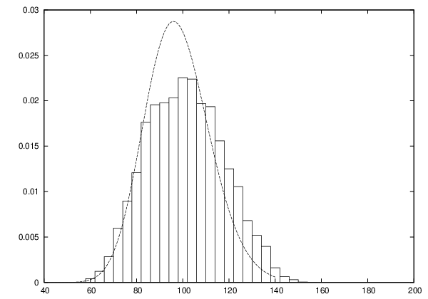

Complete independence model () Group-wise independence model ()
5.2 The analysis of PTGDR (prostanoid DP receptor) diplotype frequencies data
Next we give a numerical example of genome data. Table 3 shows diplotype frequencies on the three loci, T-549C (locus 1), C-441T (locus 2) and T-197C (locus 3) in the human genome 14q22.1, which is given in Oguma et al. (2004). Though the data is used for the genetic association studies in Oguma et al. (2004), we simply consider fitting our models. As an example, we only consider the diplotype data of patients in the population of blacks ().
| Diplotype | Whites | Blacks | ||
|---|---|---|---|---|
| Controls | Patients | Controls | Patients | |
| CCT/CCT | 16 | 78 | 7 | 10 |
| CCT/TTT | 27 | 106 | 12 | 27 |
| CCT/TCT | 48 | 93 | 4 | 12 |
| CCT/CCC | 17 | 45 | 3 | 9 |
| TTT/TTT | 9 | 43 | 2 | 7 |
| TTT/TCT | 34 | 60 | 8 | 6 |
| TTT/CCC | 4 | 28 | 1 | 6 |
| TCT/TCT | 11 | 20 | 7 | 0 |
| TCT/CCC | 6 | 35 | 1 | 2 |
| CCC/CCC | 1 | 8 | 0 | 0 |
First we consider the analysis of genotype frequency data. Though Table 3 is diplotype frequency data, here we ignore the information on the haplotypes and simply treat it as a genotype frequency data. Since and , there are distinct set of genotypes, i.e., , while only distinct haplotypes appear in Table 3. Table 4 is the set of genotype frequencies of patients in the population of blacks.
| locus 3 | CC | CT | TT | |||||||
| locus 2 | CC | CT | TT | CC | CT | TT | CC | CT | TT | |
| locus 1 | CC | 0 | 0 | 0 | 9 | 0 | 0 | 10 | 0 | 0 |
| CT | 0 | 0 | 0 | 2 | 6 | 0 | 12 | 27 | 0 | |
| TT | 0 | 0 | 0 | 0 | 0 | 0 | 0 | 6 | 7 | |
Under the genotype-wise independence model (6), the sufficient statistic is the genotype frequency data for each locus. On the other hand, under the Hardy-Weinberg model (7), the sufficient statistic is the allele frequency data for each locus, and the genotype frequencies for each locus are estimated by the Hardy-Weinberg law. Accordingly, the maximum likelihood estimates for the combination of the genotype frequencies are calculated as Table 5.
| locus 3 | CC | CT | TT | |||||||
|---|---|---|---|---|---|---|---|---|---|---|
| locus 2 | CC | CT | TT | CC | CT | TT | CC | CT | TT | |
| locus 1 | CC | 0.1169 | 0.1180 | 0.0298 | 1.939 | 1.958 | 0.4941 | 8.042 | 8.118 | 2.049 |
| 0 | 0 | 0 | 1.708 | 2.018 | 0.3623 | 6.229 | 7.361 | 1.321 | ||
| CT | 0.2008 | 0.2027 | 0.0512 | 3.331 | 3.362 | 0.8486 | 13.81 | 13.94 | 3.519 | |
| 0 | 0 | 0 | 4.225 | 4.993 | 0.8962 | 15.41 | 18.21 | 3.268 | ||
| TT | 0.0862 | 0.0870 | 0.0220 | 1.430 | 1.444 | 0.3644 | 5.931 | 5.988 | 1.511 | |
| 0 | 0 | 0 | 1.169 | 1.381 | 0.2479 | 4.262 | 5.037 | 0.9040 | ||
The configuration for the Hardy-Weinberg model is written as
and the configuration for the genotype-wise independence model is written as
Since these two configurations are of the Segre-Veronese type, again we can easily perform MCMC sampling as discussed in Section 4. After burn-in steps, we construct Monte Carlo samples. Figure 2 shows histograms of the Monte Carlo sampling generated from the exact conditional distribution of the Pearson goodness-of-fit statistics for the PTGDR genotype frequency data under the Hardy-Weinberg model and the genotype-wise independence model, respectively, along with the corresponding asymptotic distributions and .
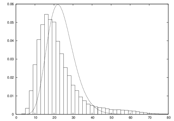
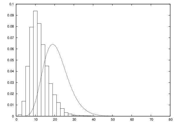
Hardy-Weinberg model () Genotype-wise independence model ()
From the Monte Carlo samples, we can also estimate the -values for each null model. The values of the Pearson goodness-of-fit for the PTGDR genotype frequency data of Table 4 are under the Hardy-Weinberg models, whereas under the genotype-wise independence model. These values are highly significant ( for both models), which implies the susceptibility of the particular haplotypes.
Next we consider the analysis of the diplotype frequency data. In this case of and , there are distinct haplotypes, and there are
distinct diplotypes, while there are only haplotypes and diplotypes appear in Table 3. The numbers of each haplotype are calculated as the second column of Table 6. Under the Hardy-Weinberg model, the haplotype frequencies are estimated proportionally to the allele frequencies, which is shown as the third column of Table 6.
| Haplotype | observed | MLE under HW | Haplotype | observed | MLE under HW |
|---|---|---|---|---|---|
| CCC | 17 | 6.078 | TCC | 0 | 5.220 |
| CCT | 68 | 50.410 | TCT | 20 | 43.293 |
| CTC | 0 | 3.068 | TTC | 0 | 2.635 |
| CTT | 0 | 25.445 | TTT | 53 | 21.853 |
The maximum likelihood estimates of the diplotype frequencies under the Hardy-Weinberg model are calculated from the maximum likelihood estimates for each haplotype. These values coincide with appropriate fractions of the values for the corresponding combination of the genotypes in Table 5. For example, the MLE for the diplotype CCT/CCT coincides with the MLE for the combination of the genotypes (CC,CC,TT) in Table 5, whereas the MLE’s for the diplotype CCC/TTT, CCT/TTC, CTC/TCT, CTT/TCC coincide with the fraction of the MLE for the combination of the genotypes (CT,CT,CT), and so on. Since we know that the Hardy-Weinberg model is highly statistically rejected, it is natural to consider the haplotype-wise Hardy-Weinberg model given in Section 3.3.2. Table 7 shows the maximum likelihood estimates under the haplotype-wise Hardy-Weinberg model. It should be noted that the MLE for the other diplotypes are all zeros.
| Diplotype | observed | MLE | Diplotype | observed | MLE |
|---|---|---|---|---|---|
| CCT/CCT | 10 | 14.6329 | TTT/TCT | 6 | 6.7089 |
| CCT/TTT | 27 | 22.8101 | TTT/CCC | 6 | 5.7025 |
| CCT/TCT | 12 | 8.6076 | TCT/TCT | 0 | 1.2658 |
| CCT/CCC | 9 | 7.3165 | TCT/CCC | 2 | 2.1519 |
| TTT/TTT | 7 | 8.8892 | CCC/CCC | 0 | 0.9146 |
We perform the Markov chain Monte Carlo sampling for the haplotype-wise Hardy-Weinberg model. The configuration for this model is written as
which is obviously of the Segre-Veronese type. We give a histogram of the Monte Carlo sampling generated from the exact conditional distribution of the Pearson goodness-of-fit statistics for the PTGDR diplotype frequency data under the haplotype-wise Hardy-Weinberg model, along with the corresponding asymptotic distributions in Figure 3.
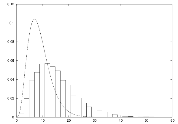
The -value for this model is estimated as with the estimated standard deviation (We also discard the first samples, and use a batching method to obtain an estimate of variance, see Hastings (1970) and Ripley (1987)). Note that the asymptotic -value based on is .
6 Some discussions
In this paper we considered independence models in group-wise selections, which can be described in terms of a Segre-Veronese configuration. We have shown that our framework can be applied to two important examples in educational statistics and biostatistics. We expect that the methodology of the present paper finds applications in many other fields.
In the NCT example, we assumed that the examinees choose the same number of subjects. We also assumed for simplicity that the examinees choose either nothing or one subject from a subgroup. This restricts our analysis to some subset of the examinees of NCT. Actually the examinees make decisions on how many subjects to take and modeling this decision making is clearly of statistical interest. Further complication arises from the fact that the examinees can choose which scores to submit to universities after taking NCT. For example after obtaining scores of three subjects on Science, an examinee can choose the best two scores for submitting to a university. In our subsequent paper (Aoki et al., 2007) we present a generalization of Segre-Veronese configurations to cope with these complications.
It seems that the simplicity of the reduced Gröbner basis for the Segre-Veronese configuration comes from the fact that the index set of the rows of can be ordered and the restriction on the counts can be expressed in terms of one-dimensional intervals. From statistical viewpoint, ordering of the elements of the sufficient statistic in group-wise selection seems to be somewhat artificial. It is of interest to look for other statistical models, where ordering of the elements of the sufficient statistic is more natural and the Segre-Veronese configuration can be applied.
References
- Aoki et al. (2007) Aoki, S., Hibi, T., Ohsugi, H. and Takemura, A. (2007). Gröbner bases of nested configurations. Submitted for publication.
- Aoki and Takemura (2005) Aoki, S. and Takemura, A. (2005). Markov chain Monte Carlo exact tests for incomplete two-way contingency tables. Journal of Statistical Computation and Simulation. 75, 787–812.
- Aoki and Takemura (2006) Aoki, S. and Takemura, A. (2006). Markov chain Monte Carlo tests for designed experiments. arXiv:math/0611463v1. Submitted for publication.
- Aoki and Takemura (2007) Aoki, S. and Takemura, A. (2007). Minimal invariant Markov basis for sampling contingency tables with fixed marginals. Annals of the Institute of Statistical Mathematics, To appear.
- (5) Beerenwinkel, N., Eriksson, N. and Sturmfels, B. (2006). Conjunctive Bayesian networks. arXiv:math/0608417v3. To appear in Bernoulli.
- (6) Bishop, Y. M. M., Fienberg, S. E. and Holland P. W. (1975). Discrete Multivariate Analysis: Theory and Practice. The MIT Press, Cambridge, Massachusetts.
- Crow (1988) Crow, J. E. (1988). Eighty years ago: The beginnings of population genetics. Genetics, 119, 473–476.
- (8) De Negri, E. and Hibi, T. (1997). Gorenstein algebras of Veronese type. Journal of Algebra, 193, no. 2, 629–639.
- Diaconis and Sturmfels (1998) Diaconis, P. and Sturmfels, B. (1998). Algebraic algorithms for sampling from conditional distributions. The Annals of Statistics, 26, 363–397.
- (10) Guo, S. and Thompson, E. (1992). Performing the exact test of Hardy-Weinberg proportion for multiple alleles. Biometrics, 48, 361–372.
- Hastings (1970) Hastings, W. K. (1970). Monte Carlo sampling methods using Markov chains and their applications. Biometrika, 57, 97–109.
- (12) Hibi, T. (1987). Distributive lattices, affine semigroup rings and algebras with straightening laws. Advanced Studies in Pure Mathematics, 11, 93–109.
- (13) Huber, M., Chen, Y., Dinwoodie, I., Dobra, A. and Nicholas, M. (2006). Monte Carlo algorithms for Hardy-Weinberg proportions. Biometrics, 62, 49–53.
- Lehmann (1986) Lehmann, E. L. and Romano, J. P. (2005). Testing Statistical Hypotheses, 3rd ed. Springer, New York.
- (15) National Center for University Entrance Examinations. (2006). Booklet on NCUEE. Available from http://www.dnc.ac.jp/dnc/gaiyou/pdf/youran_english_H18_HP.pdf
- (16) Oguma, T., Palmer, L. J., Birben, E., Sonna, L. A. Asano, K. and Lilly, C. M. (2004). Role of prostanoid DP receptor variants in susceptibility to asthma. The New England Journal of Medicine, 351, 1752–1763.
- (17) Ohsugi, H. and Hibi, T. (2000). Compressed polytopes, initial ideals and complete multipartite graphs, Illinois Journal of Mathematics, 44, 391–406.
- Ohsugi and Hibi (2005) Ohsugi, H. and Hibi, T. (2005). Indispensable binomials of finite graphs. Journal of Algebra and Its Applications, 4, 421–434.
- (19) Ohsugi, H. and Hibi, T. (2006). Quadratic Gröbner bases arising from combinatorics. Integer Points in Polyhedra - Geometry, Number Theory, Representation Theory, Algebra, Optimization, Statistics, To appear.
- (20) Ohsugi, H. and Hibi, T. (2007). Toric ideals arising from contingency tables. in “Commutative Algebra and Combinatorics,” Ramanujan Mathematical Society Lecture Notes Series, Number 4, Ramanujan Mathematical Society, India, in press.
- (21) Pachter, L. and Sturmfels, B. (2005). Algebraic Statistics for Computational Biology. Cambridge University Press, Cambridge.
- (22) Rapallo, F. (2006). Markov bases and structural zeros. Journal of Symbolic Computation, 41, 164–172.
- Ripley (1987) Ripley, B. D. (1987). Stochastic Simulation. Wiley, New York.
- Sturmfels (1995) Sturmfels, B. (1995). Gröbner Bases and Convex Polytopes. American Mathematical Society, Providence, RI.
- Takemura and Aoki (2004) Takemura, A. and Aoki, S. (2004). Some characterizations of minimal Markov basis for sampling from discrete conditional distributions. Annals of the Institute of Statistical Mathematics, 56, 1–17.
Appendix A Tables of numbers of examinees in NCT in 2006
| Geography and History | Civics | # total | # actual | ||||||||
| WHA | WHB | JHA | JHB | GeoA | GeoB | ContS | Ethics | P&E | examinees | examinees | |
| 1 subject | 496 | 29,108 | 1,456 | 54,577 | 1,347 | 27,152 | 40,677 | 16,607 | 25,321 | 196,741 | 196,741 |
| 2 subjects | 1,028 | 61,132 | 3,386 | 90,427 | 5,039 | 83,828 | 180,108 | 27,064 | 37,668 | 489,680 | 244,840 |
| Total | 1,524 | 90,240 | 4,842 | 145,004 | 6,386 | 110,980 | 220,785 | 43,671 | 62,989 | 686,421 | 441,581 |
| Geography and History | |||||||
| Civics | WHA | WHB | JHA | JHB | GeoA | GeoB | Total |
| ContSoc | 687 | 39,913 | 2,277 | 62,448 | 3,817 | 70,966 | 180,108 |
| Ethics | 130 | 10,966 | 409 | 10.482 | 405 | 4,672 | 27,064 |
| P&E | 211 | 10253 | 700 | 17,497 | 817 | 8,190 | 37,668 |
| Total | 1,028 | 61,132 | 3,386 | 90,427 | 5,039 | 83,838 | 244,840 |
| Science 1 | Science 2 | Science 3 | # total | #actual | |||||||||
| CSciB | BioI | ISci | BioIA | CSciA | ChemI | ChemIA | PhysI | EarthI | PhysIA | EarthIA | examinees | examinees | |
| 1 subject | 2,558 | 80,385 | 511 | 1,314 | 1,569 | 19,616 | 717 | 14,397 | 10,788 | 289 | 236 | 132,380 | 132,380 |
| 2 subjects | 6,878 | 79,041 | 523 | 1,195 | 26,848 | 158,027 | 2,777 | 106,822 | 6,913 | 905 | 259 | 390,188 | 195,094 |
| 3 subjects | 7,942 | 18,519 | 728 | 490 | 6,838 | 20,404 | 437 | 18,451 | 8,423 | 361 | 444 | 83,037 | 27,679 |
| Total | 17,378 | 177,945 | 1,762 | 2,999 | 35,255 | 198,047 | 3,931 | 139,670 | 26,124 | 1,555 | 939 | 605,605 | 355,153 |
| Science | Science | |||||||
| CSciA | ChemI | ChemIA | PhysI | EarthI | PhysIA | EarthIA | ||
| Science 1 | CSciB | 1,501 | 1,334 | 23 | 120 | 3,855 | 1 | 44 |
| BioI | 21,264 | 54,412 | 244 | 1,366 | 1,698 | 5 | 52 | |
| ISci | 147 | 165 | 50 | 43 | 92 | 5 | 21 | |
| BioIA | 128 | 212 | 715 | 16 | 33 | 29 | 62 | |
| Science 3 | Physics | 3,243 | 101,100 | 934 | — | — | — | — |
| EarthI | 485 | 730 | 20 | — | — | — | — | |
| PhysIA | 43 | 54 | 768 | — | — | — | — | |
| EarthIA | 37 | 20 | 23 | — | — | — | — | |
| Science | PhysI | EarthI | Physics IA | Earth science IA | |||||||||
| Science | CSciA | ChemI | ChemIA | CSciA | ChemI | ChemIA | CSciA | ChemI | ChemIA | CSciA | ChemI | ChemIA | |
| Science | CSciB | 1,155 | 5,152 | 17 | 1,201 | 317 | 7 | 16 | 5 | 16 | 48 | 5 | 3 |
| BioI | 553 | 10,901 | 31 | 3,386 | 3,342 | 16 | 30 | 35 | 19 | 130 | 56 | 20 | |
| ISci | 80 | 380 | 23 | 62 | 34 | 4 | 32 | 13 | 27 | 48 | 14 | 11 | |
| BioIA | 6 | 114 | 39 | 22 | 22 | 10 | 12 | 6 | 150 | 57 | 8 | 44 | |