Upper bounds on entangling rates of bipartite Hamiltonians

Consider two remote parties Alice and Bob controlling finite-dimensional quantum systems $A$ and $B$. Suppose $A$ and $B$ interact with each other according to a time-independent Hamiltonian $H$. Unless $H$ is a sum of local Hamiltonians, a unitary evolution $e^{iHt}$ is a non-local operation capable of creating entanglement between $A$ and $B$. The goal of the present paper is to get an upper bound on the rate at which the entanglement between Alice and Bob can increase or decrease as a function of time.

We consider ancilla-assisted entangling, see Figure 1. It means that Alice’s laboratory consists of two subsystems: $A$ and $a$, such that the Hamiltonian $H$ acts only on the subsystem $A$. Similarly, Bob’s laboratory is partitioned into $B$ and $b$, where $H$ acts only on the subsystem $B$. The subsystems $a$ and $b$ are the local ancillas held by Alice and Bob. In the ancilla-assisted entangling Alice and Bob start from a pure state $|\Psi\rangle$ of the composite system $aABb$ which may be already entangled.

Time evolution of the composite system $aABb$ is described by a unitary operator $U(t)=I_{a}\otimes e^{iH_{AB}t}\otimes I_{b}$. Thus the joint state of Alice and Bob always remains pure. Accordingly, the entanglement between Alice and Bob at any time $t$ can be quantified by entanglement entropy

$$S(aA)=-\mathop{\mathrm{Tr}}\nolimits{\rho_{aA}(t)\,\log{\rho_{aA}(t)}},\quad\rho_{aA}(t)=\mathop{\mathrm{Tr}}\nolimits_{Bb}U(t)\,|\Psi\rangle\langle\Psi|\,U(t)^{\dagger}.$$

(1)

The quantity we are interested in is entangling rate

$$\Gamma(\Psi,H)=\left.\frac{dS(aA)}{dt}\right|_{t=0}.$$

(2)

Understanding properties of the entangling rate is crucial for optimal generation of entanglement [1], computing capacities of bidirectional quantum communication channels [2], and for describing dynamics of entanglement in quantum spin lattice models [3].

Our goal is to get an upper bound on $\Gamma(\Psi,H)$ that would not explicitly depend upon dimensions of the local ancillas $a$ and $b$. Upper bounds of this kind can be easily generalized via the Trötter decomposition to arbitrary multipartite Hamiltonians decomposable into a sum of few-party interactions.

The maximal entangling rate can be easily found in the absence of local ancillas, i.e., when $a=b=1$. In this case we can always write the initial state of Alice and Bob using the Schmidt decomposition $|\Psi\rangle=\sum_{j=1}^{d}\sqrt{p_{j}}\,|j_{A}\rangle\otimes|j_{B}\rangle$ with $d=\min{(A,B)}$. Denote $\rho_{A}=\sum_{j=1}^{d}p_{j}\,|j\rangle\langle j|$ the reduced density matrix of Alice. Using the general formula Eq. (4) for the entangling rate one gets

$$\Gamma(\Psi,H)=-\mathop{\mathrm{Tr}}\nolimits{\dot{\rho_{A}}\,\log{\rho_{A}}}=-i\mathop{\mathrm{Tr}}\nolimits{\left(H\,[\,|\Psi\rangle\langle\Psi|,\log{\rho_{A}}\otimes I_{B}\,]\right)}.$$

(8)

Since the entangling rate is a linear function of $H$ we can assume that $\|H\|=1$. Using the fact that for any Hermitian operator $X$

$$\max_{H\,:\|H\|=1}\mathop{\mathrm{Tr}}\nolimits{(H\,X)}=\mathop{\mathrm{Tr}}\nolimits{|X|}\equiv\|X\|_{1},$$

(9)

one can carry out the maximization over $H$,

$$\Gamma(\Psi):=\max_{H\,:\,\|H\|=1}\Gamma(\Psi,H)=\|\;\;[\,\log{\rho_{A}}\otimes I_{B},|\Psi\rangle\langle\Psi|\,]\;\;\|_{1}.$$

(10)

For any vectors $|\Psi\rangle,|\Phi\rangle$ one has the following identity

$$\|\;|\Phi\rangle\langle\Psi|-|\Psi\rangle\langle\Phi|\;\|_{1}=2\sqrt{\langle\Psi|\Psi\rangle\langle\Phi|\Phi\rangle-|\langle\Psi|\Phi\rangle|^{2}}.$$

(11)

Substituting $|\Phi\rangle=(\log{\rho_{A}}\otimes I_{B})\,|\Psi\rangle$ one gets

$$\Gamma(\Psi)=2\sqrt{F(p)},\quad F(p):=\sum_{j=1}^{d}p_{j}\,\mathrm{log}^{2}{p_{j}}-\left(\sum_{j=1}^{d}p_{j}\,\log{p_{j}}\right)^{2}.$$

(12)

We can assume that all $p_{j}>0$ (otherwise replace $d$ by $d^{\prime}<d$). Then the maximum of $F(p)$ can be found by solving extremal point equations $\partial F/\partial p_{j}=0$. After simple algebra one gets

$$-\log{(2p_{j})}=S\pm\sqrt{\gamma^{2}+S^{2}},\quad S=-\sum_{j=1}^{d}p_{j}\,\log{p_{j}},\quad\gamma=\frac{1}{\ln{2}}.$$

(13)

(Here $\log$ and $\ln$ stand for base two and natural logarithm.) The equality for the minus sign in the r.h.s. of Eq. (13) is possible only for one value of $j$, since it implies $p_{j}\geq 1/2$. Let us agree that $p_{1}\geq 1/2$. Then $-\log{(2p_{j})}=S+\sqrt{\gamma^{2}+S^{2}}$ for all $j=2,\ldots,d$, that is the state $\rho_{A}$ must have a binary spectrum with multiplicities $1,d-1$. Introduce a variable $\lambda$ such that

$$p_{1}=\lambda,\quad p_{2}=\ldots=p_{d}=\frac{1-\lambda}{d-1},\quad\frac{1}{2}\leq\lambda\leq 1.$$

(14)

Let $|\Psi_{\lambda}\rangle$ be the state with Schmidt coefficients $p_{1},\ldots,p_{d}$. Using Eq. (12) the maximal entangling rate with the initial state $|\Psi_{\lambda}\rangle$ can be written as

$$\Gamma(\Psi_{\lambda})=2\sqrt{\lambda(1-\lambda)}\log{\left(\frac{\lambda(d-1)}{1-\lambda}\right)}.$$

(15)

The optimal value $\lambda=\lambda(d)$ and the optimal entangling rate $\Gamma_{d}=\Gamma(\Psi_{\lambda(d)})$ have to be found by maximizing Eq. (15) over $1/2\leq\lambda\leq 1$. For example, if $d=2$, numerical maximization yields $\lambda(2)\approx 0.9168$ and $\Gamma_{2}\approx 1.9123$. It coincides with the maximal entangling rate of product two-qubit Hamiltonians found in [1, 4]. It follows that under normalization condition $\|H\|=1$ product two-qubit Hamiltonians are capable of generating entanglement with the largest rate.

One can easily infer from Eq. (15) that $\lambda(d)\approx 1/2$ and $\Gamma_{d}\approx\log{d}$ for sufficiently large $d$. It proves that $\Gamma(\Psi,H)=O(\|H\|\log{d})$ in the absence of local ancillas. Moreover, in the limit of large $d$ one can explicitly write down the optimal state $|\Psi_{\lambda(d)}\rangle$ and the optimal Hamiltonian $H_{d}$. Namely,

$$|\Psi_{\lambda(d)}\rangle\approx\frac{1}{\sqrt{2}}\,|1\rangle\otimes|1\rangle+\frac{1}{\sqrt{2}}\,|\Phi^{+}\rangle,\quad|\Phi^{+}\rangle=\frac{1}{\sqrt{d-1}}\sum_{j=2}^{d}|j\rangle\otimes|j\rangle,$$

(16)

$$H_{d}\approx-i(\,|\Phi^{+}\rangle\langle 1,1|-|1,1\rangle\langle\Phi^{+}|\,).$$

(17)

Thus the optimal state is a superposition of a product state and a maximally entangled state with locally orthogonal supports. The optimal Hamiltonian is a generator for a rotation in the corresponding two-dimensional subspace.

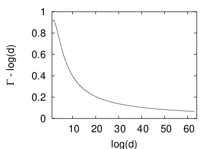
For a finite $d$ the optimal value $\lambda(d)$ and the corresponding entangling rate $\Gamma_{d}$ can be found numerically, see Figure 2. For large $d$ one has $\lambda(d)\approx(1/2)(1+1/\ln{d})$, while entanglement entropy of $|\Psi_{\lambda(d)}\rangle$ scales as $S_{d}\approx(1/2)\,\log{d}$.

In this section we assume that SIM is true and show that this assumption implies SIE. Consider ancilla-assisted entangling with dimensions $a,A,B,b$ and some initial state $|\Psi\rangle$. Let us assume that $B\leq A$. Then SIE is equivalent to an upper bound

$$\Gamma(\Psi,H)\leq c\|H\|\log{B}.$$

(18)

Since the r.h.s. of this inequality does not depend on $a$ and $A$, it is enough to prove Eq. (18) in the case $a=1$ since we can always extend $A$ to $A\otimes a$. Now we have a tripartite system $ABb$ initially prepared in a pure state $|\Psi\rangle$ and evolving under a Hamiltonian $H$ acting on $A$ and $B$. Using formula Eq. (4) for the entangling rate one gets

$$\Gamma(\Psi,H)=-i\mathop{\mathrm{Tr}}\nolimits{\left(H\,[\,\rho_{AB},\log{\rho_{A}}\otimes I_{B}\,]\right)}=-i\mathop{\mathrm{Tr}}\nolimits{\left(H\,[\,\rho_{AB},\log{\tau_{AB}}\,]\right)},$$

(19)

where $\rho_{A}$ and $\rho_{AB}$ are the reduced states of $|\Psi\rangle$, and a state $\tau_{AB}$ is defined as

$$\tau_{AB}=\rho_{A}\otimes\frac{I_{B}}{B}.$$

(20)

In order to define a probabilistic ensemble ${\cal E}$ needed for a reduction to SIM we shall need the following lemma.

Proof: Since the partial trace is a linear operation, it suffices to prove the lemma for the case when $\rho_{AB}=|\psi\rangle\langle\psi|$ is a pure state. The statement of the lemma is then equivalent to inequality

$$|\psi\rangle\langle\psi|\leq B\,\rho_{A}\otimes I_{B}.$$

(22)

Let $d$ be the Schmidt rank of $|\psi\rangle$. Obviously, $d\leq\min{(A,B)}$. Consider a state $|I\rangle=\sum_{j=1}^{d}|j_{A}\rangle\otimes|j_{B}\rangle$, where $\{|j_{A}\rangle\}$ and $\{|j_{B}\rangle\}$ are the local bases of $A$ and $B$ that diagonalize $\rho_{A}$ and $\rho_{B}$. Then

$$|\psi\rangle\langle\psi|=(\rho_{A}^{\frac{1}{2}}\otimes I_{B})\,|I\rangle\langle I|\,(\rho_{A}^{\frac{1}{2}}\otimes I_{B}).$$

Taking into account that $\langle I|I\rangle=d$, one concludes that $|I\rangle\langle I|\leq d\,I_{AB}$. Multiplying this inequality by $\rho_{A}^{\frac{1}{2}}\otimes I_{B}$ on the left and on the right we get $|\psi\rangle\langle\psi|\leq d\,\rho_{A}\otimes I_{B}$ which implies Eq. (22).

$\Box$

Define an ensemble of states ${\cal E}=\{p_{\alpha},\tau_{\alpha}\}_{\alpha=0,1}$ such that $\tau_{0}=\mu_{AB}$, $\tau_{1}=\rho_{AB}$, $p_{0}=1-B^{-2}$, $p_{1}=B^{-2}$. Here $\mu_{AB}$ is the state that appears in the decomposition Eq. (21). This ensemble has the average state $\tau=p_{0}\,\tau_{0}+p_{1}\,\tau_{1}=\rho_{A}\otimes I_{B}/B$. Let $H$ be a Hamiltonian that appears in Eq. (19). Assuming that SIM is true one gets

$$\Lambda({\cal E},H)\leq c^{\prime}\,h(B^{-2},1-B^{-2})\,\|H\|\leq 4c^{\prime}B^{-2}\,\log{B}\,\|H\|.$$

(23)

(Note that for any $x\leq 1/2$ one has $h(x,1-x)\leq 2x|\log{x}|$.) On the other hand, formula Eq. (7) for the mixing rate leads to

$$\Lambda({\cal E},H)=-ip_{1}\mathop{\mathrm{Tr}}\nolimits{\left(H\,[\;\tau_{1},\log{\tau}\;]\right)}=-iB^{-2}\mathop{\mathrm{Tr}}\nolimits{\left(H\,[\;\rho_{AB},\log{\tau_{AB}}\;]\right)}.$$

(24)

Combining Eqs. (23,24) one arrives to

$$-i\mathop{\mathrm{Tr}}\nolimits{\left(H\,[\;\rho_{AB},\log{\tau_{AB}}\;]\right)}\leq 4c^{\prime}\,\log{B}\,\|H\|.$$

Comparing it with Eq. (19) we infer that $\Gamma(\Psi,H)\leq 4c^{\prime}\,\log{B}\,\|H\|$. We have proved SIE with a constant $c=4c^{\prime}$, see Eq. (18).

The reduction Eq. (20) has a peculiar property that the number of distinct eigenvalues of $\tau_{AB}$ and $\rho_{A}$ are the same. Since we have used identification $A=aA$, the number of distinct eigenvalues of $\rho_{A}$ coincides with the number of distinct Schmidt coefficients of $|\Psi\rangle$. Thus if we can prove SIM with $\rho(0)$ having only two distinct eigenvalues, we will prove SIE for the case when $|\Psi\rangle$ has only two distinct Schmidt coefficients.

Let us start from proving a weaker (compared to SIM) upper bound on the mixing rate.

Proof: Suppose ${\cal E}=\{p_{\alpha},\rho_{\alpha}\}_{\alpha=0,1}$, where the states $\rho_{0},\rho_{1}$ and a Hamiltonian $H$ are defined on a $D$-dimensional Hilbert space. Consider ancilla-assisted entangling protocol shown on Figure 1 with $a=1$, $A=D$, $B=2$, $b=D$. Choose a Hamiltonian $\tilde{H}$ coupling $A$ and $B$ as

$$\tilde{H}=H_{A}\otimes|1\rangle\langle 1|_{B}.$$

Choose the initial state as

$$|\Psi\rangle=\sqrt{p_{0}}\,|0\rangle_{B}\otimes|\phi_{0}\rangle_{Ab}+\sqrt{p_{1}}\,|1\rangle_{B}\otimes|\phi_{1}\rangle_{Ab},$$

where $|\phi_{\alpha}\rangle\in\mathbb{C}^{D}\otimes\mathbb{C}^{D}$ is a purification of $\rho_{\alpha}$. Then the state $|\Psi\rangle$ evolves in time as

$$|\Psi(t)\rangle=\sqrt{p_{0}}\,|0\rangle_{B}\otimes|\phi_{0}\rangle_{Ab}+\sqrt{p_{1}}\,|1\rangle_{B}\otimes(e^{iH_{A}t}\otimes I_{b})\,|\phi_{1}\rangle_{Ab}.$$

Accordingly, $\rho_{A}(t)=p_{0}\,\rho_{0}+p_{1}\,e^{iHt}\rho_{1}e^{-iHt}$. Therefore $\Lambda({\cal E},H)=\Gamma(\Psi,\tilde{H})$. Now we can use the upper bound on the entangling rate obtained in [6, 7] for product Hamiltonians, namely $\Gamma(\Psi,\tilde{H})\leq\beta\,\|\tilde{H}\|=\beta\,\|H\|$, where $\beta\approx 1.9123\leq 2$. The lemma is proved.

$\Box$

This lemma implies that the whole difficulty of proving SIM (if it is true) concerns the limiting cases $p_{0}\to 0$ or $p_{0}\to 1$. Note also that $\Lambda({\cal E},H)=\Lambda({\cal E}^{T},-H)$, where ensemble ${\cal E}^{T}$ is obtained from ${\cal E}$ by interchanging $p_{0},\rho_{0}$ with $p_{1},\rho_{1}$. Thus we can assume that $0\leq p_{1}\leq 1/2$.

In the following we shall represent an ensemble ${\cal E}=\{p_{\alpha},\rho_{\alpha}\}_{\alpha=0,1}$ using the data $(p,\rho,\Pi)$, where

$$p=p_{1},\quad\rho=(1-p)\,\rho_{0}+p\,\rho_{1},\quad\Pi=p\,\rho^{-\frac{1}{2}}\,\rho_{1}\,\rho^{-\frac{1}{2}}.$$

(26)

One can easily check that a triple $(p,\rho,\Pi)$ represents some ensemble ${\cal E}$ iff

$$0\leq p\leq 1,\quad 0\leq\Pi\leq I,\quad\mathop{\mathrm{Tr}}\nolimits{\Pi\rho}=p.$$

(27)

Indeed, the only non-trivial statement is that $\Pi\leq I$. It can be obtained from inequality $p_{1}\,\rho_{1}\leq\rho$ by multiplying it by $\rho^{-1/2}$ on the left and on the right. Using the representation Eq. (26) one can rewrite the mixing rate as

$$\Lambda({\cal E},H)=-i\mathop{\mathrm{Tr}}\nolimits{\left(H\,\rho^{\frac{1}{2}}\,[\;\Pi,\log{\rho}\;]\,\rho^{\frac{1}{2}}\right)},$$

(28)

see Eq. (7). Given ${\cal E}$, the optimal Hamiltonian $H$ maximizing the mixing rate can be found using Eq. (9). Thus we have

$$\Lambda({\cal E}):=\max_{H\,:\|H\|=1}\Lambda({\cal E},H)=\|\,\rho^{\frac{1}{2}}\,[\;\Pi,\log{\rho}\;]\,\rho^{\frac{1}{2}}\,\|_{1}.$$

(29)

It is worth mentioning that for given $\rho$ the upper bound Eq. (6) is true for sufficiently small $p$. Indeed, applying the triangle inequality for the trace norm to Eq. (29) one gets $\Lambda({\cal E})\leq 2\|\,\rho^{\frac{1}{2}}\Pi\rho^{\frac{1}{2}}\,\log{\rho}\,\|_{1}$. Since $\|\,AB\,\|_{1}\leq\|A\|\,\|B\|_{1}$ for any operators $A,B$ it follows that $\Lambda({\cal E})\leq 2\|\log{\rho}\|\|\,\rho^{\frac{1}{2}}\Pi\rho^{\frac{1}{2}}\,\|_{1}$. If $p$ is smaller than the smallest eigenvalue of $\rho$, one has $\|\log{\rho}\|\leq|\log{p}|$ and thus $\Lambda({\cal E})\leq 2|\log{p}|\mathop{\mathrm{Tr}}\nolimits{(\Pi\rho)}=2p|\log{p}|\leq 2h(p,1-p)$.

In the rest of the section we prove SIM under the assumption that $\rho$ has binary spectrum,

$$\rho=\sum_{j=1}^{D}\rho_{j}\,|j\rangle\langle j|,\quad\rho_{j}=\left\{\begin{array}[]{rcl}\lambda_{1}&\mbox{if}&j=1,\ldots,m\\ \lambda_{2}&\mbox{if}&j=m+1,\ldots,D,\\ \end{array}\right.,\quad\lambda_{1}\geq\lambda_{2}.$$

Here $m$ can be arbitrary integer between $1$ and $D$. Define projectors $R=\sum_{j=1}^{m}|j\rangle\langle j|$ and $R^{\perp}=I-R$ such that

$$\rho=\lambda_{1}\,R+\lambda_{2}\,R^{\perp},\quad\rho^{\frac{1}{2}}=\sqrt{\lambda_{1}}\,R+\sqrt{\lambda_{2}}\,R^{\perp},\quad\log{\rho}=\log{\lambda_{1}}\,R+\log{\lambda_{2}}\,R^{\perp}.$$

After some algebra one gets the following identity

$$\rho^{\frac{1}{2}}\,[\;\Pi,\log{\rho}\;]\,\rho^{\frac{1}{2}}=\log{\left(\frac{\lambda_{1}}{\lambda_{2}}\right)}\,\sqrt{\lambda_{1}\,\lambda_{2}}\,[\;\Pi,R\;].$$

(30)

In order to upper bound the trace norm of the commutator $[\Pi,R]$ we shall use the following.

We shall postpone the proof of the two lemmas above until the end of the section. Let us apply Lemma 3 to the commutator in Eqs. (30) where $\Pi$ is replaced by $\Pi^{\prime}$ from Lemma 4. Then we can upper bound the mixing rate in Eq. (29) as

$$\Lambda({\cal E})\leq 2\log{\left(\frac{\lambda_{1}}{\lambda_{2}}\right)}\,\sqrt{\lambda_{1}\,\lambda_{2}\,\mathop{\mathrm{Tr}}\nolimits{(\Pi^{\prime}\,R)}\,\mathop{\mathrm{Tr}}\nolimits{(\Pi^{\prime}\,R^{\perp})}}.$$

(32)

In order to analyze the expression above introduce new variables $m^{\prime},p^{\prime},x_{1},x_{2}$ such that

$$m^{\prime}=\mathop{\mathrm{Tr}}\nolimits{\Pi^{\prime}},\quad p^{\prime}=\mathop{\mathrm{Tr}}\nolimits{(\Pi^{\prime}\rho)},\quad x_{i}=\lambda_{i}\,m^{\prime}.$$

(33)

Expressing $\mathop{\mathrm{Tr}}\nolimits{(\Pi^{\prime}\,R)}$ and $\mathop{\mathrm{Tr}}\nolimits{(\Pi^{\prime}\,R^{\perp})}$ in terms of $m^{\prime}$ and $p^{\prime}$ one can rewrite Eq. (32) as

$$\Lambda({\cal E})\leq 2\log{\left(\frac{x_{1}}{x_{2}}\right)}\,\sqrt{\frac{x_{1}\,x_{2}\,(p^{\prime}-x_{2})\,(x_{1}-p^{\prime})}{(x_{1}-x_{2})^{2}}}\equiv g(x_{1},x_{2}).$$

(34)

Let us find constraints on the variables $x_{1},x_{2}$. Noting that $\lambda_{2}\,I\leq\rho\leq\lambda_{1}\,I$ and taking the trace with $\Pi^{\prime}$ one gets $x_{2}\leq p^{\prime}\leq x_{1}$. Besides, condition (iii) of Lemma 4 implies that $m^{\prime}\leq m$ and thus $x_{1}\leq m\lambda_{1}\leq\mathop{\mathrm{Tr}}\nolimits{\rho}=1$. By obvious reasons one also has $x_{2}\geq 0$. Summarizing,

$$0\leq x_{2}\leq p^{\prime}\leq x_{1}\leq 1.$$

(35)

Now the problem of getting upper bound on the mixing rate reduces to maximizing a function $g(x_{1},x_{2})$ in Eq. (34) under constraints Eq. (35). We prove (see Lemma 5 at the end of the section) that $\max_{x_{1},x_{2}}g(x_{1},x_{2})\leq 6\,p^{\prime}|\log{p^{\prime}}|$ as long as $p^{\prime}\leq 1/2$. Using condition (i) of Lemma 4 we get $p^{\prime}=\mathop{\mathrm{Tr}}\nolimits{(\Pi^{\prime}\rho)}\leq\mathop{\mathrm{Tr}}\nolimits{(\Pi\rho)}=p$. As was mentioned in the beginning of the section, we can assume that $p\leq 1/2$ and thus $p^{\prime}\leq p\leq 1/2$. Summarizing, we get

$$\Lambda({\cal E})\leq 6\,p^{\prime}|\log{p^{\prime}}|\leq 6\,p|\log{p}|\leq 6\,h(p,1-p),$$

where we used the fact that a function $x|\log{x}|$ is monotone increasing on the interval $[0,1/2]$. Thus we have proved SIM under the assumption that $\rho$ has a binary spectrum.

Proof of Lemma 3: Hölder inequality asserts that

$$\|\,XY\,\|_{1}\leq\sqrt{\mathop{\mathrm{Tr}}\nolimits{(X^{\dagger}X)}\mathop{\mathrm{Tr}}\nolimits{(Y^{\dagger}Y)}}$$

(36)

for any operators $X$ and $Y$, see [12]. In order to choose proper $X$ and $Y$ let us use an identity $[\,\Pi,R\,]=R^{\perp}\Pi R-R\Pi R^{\perp}$ and triangle inequality for the trace norm:

$$\|\,[\;\Pi,R\;]\,\|_{1}\leq\|\,R^{\perp}\Pi R\,\|_{1}+\|\,R\Pi R^{\perp}\,\|_{1}=2\|R^{\perp}\Pi R\|_{1}=2\|\,(R^{\perp}\Pi^{\frac{1}{2}})(\Pi^{\frac{1}{2}}R)\,\|_{1}.$$

Substituting $X=R^{\perp}\Pi^{\frac{1}{2}}$ and $Y=\Pi^{\frac{1}{2}}R$ into Eq. (36) and noting that $R$, $R^{\perp}$ are projectors we get the inequality stated in the lemma.

$\Box$

Proof of Lemma 4: Any Hermitian operator $\Pi$ satisfying $0\leq\Pi\leq I$ can be written as a convex combination of projectors:

$$\Pi=\sum_{\alpha}p_{\alpha}\,\Pi_{\alpha},\quad\Pi_{\alpha}^{\dagger}\,\Pi_{\alpha}=\Pi_{\alpha}.$$

Suppose we can find the operator promised in the lemma for every projector in the sum, that is we can find $\Pi_{\alpha}^{\prime}$ such that (i) $0\leq\Pi_{\alpha}^{\prime}\leq\Pi_{\alpha}$, (ii) $[\Pi_{\alpha}^{\prime},R]=[\Pi_{\alpha},R]$, and (iii) $\mathop{\mathrm{Tr}}\nolimits{\Pi_{\alpha}^{\prime}}\leq m$. Then we can choose the desired operator $\Pi^{\prime}$ as $\Pi^{\prime}=\sum_{\alpha}p_{\alpha}\Pi_{\alpha}^{\prime}$. Thus it suffices to prove the lemma for the case when $\Pi$ is a projector. Let $D$ be the dimension of the Hilbert space. Consider a direct sum decomposition

$$\mathbb{C}^{D}={\cal H}\oplus{\cal H}^{\perp},$$

where ${\cal H}$ is the range of $R$, so that $\mbox{dim}({\cal H})=m$. Then we can write

$$R=\left(\begin{array}[]{cc}I&0\\ 0&0\\ \end{array}\right),\quad\Pi=\left(\begin{array}[]{cc}A&C\\ C^{\dagger}&B\\ \end{array}\right).$$

(37)

Here $0\leq A\leq I$ and $0\leq B\leq I$ are Hermitian operators on ${\cal H}$ and ${\cal H}^{\perp}$ and $C$ is some operator $C\,:\,{\cal H}^{\perp}\to{\cal H}$. The requirement that $\Pi$ is a projector implies

$$A\,(I-A)=CC^{\dagger},\quad B\,(I-B)=C^{\dagger}C,\quad C\,(I-B)=AC.$$

(38)

Consider a decomposition $A=A^{\prime}\oplus A^{\prime\prime}$, $B=B^{\prime}\oplus B^{\prime\prime}$ where $0<A^{\prime}<I$ and $0<B^{\prime}<I$, while $A^{\prime\prime}$ and $B^{\prime\prime}$ have only eigenvalues $0,1$. It follows from Eq. (38) that

$$A^{\prime\prime}\,CC^{\dagger}=CC^{\dagger}\,A^{\prime\prime}=0,\quad B^{\prime\prime}\,C^{\dagger}C=C^{\dagger}C\,B^{\prime\prime}=0.$$

Thus $C^{\dagger}\,|\psi\rangle=0$ for any $|\psi\rangle$ from the range of $A^{\prime\prime}$ and $C\,|\phi\rangle=0$ for any $|\phi\rangle$ from the range of $B^{\prime\prime}$. Accordingly, the projector $\Pi$ has the following block structure

$$\Pi=\left(\begin{array}[]{cccc}A^{\prime\prime}&0&0&0\\ 0&A^{\prime}&C^{\prime}&0\\ 0&(C^{\prime})^{\dagger}&B^{\prime}&0\\ 0&0&0&B^{\prime\prime}\\ \end{array}\right).$$

(39)

Let $\Pi^{\prime}$ be the central block in $\Pi$. Clearly $\Pi^{\prime}$ is a projector and $\Pi^{\prime}$ satisfies conditions (i) and (ii) of the lemma. It remains to check that $\mathop{\mathrm{Tr}}\nolimits{\Pi^{\prime}}\leq m$. Let $m^{\prime}$ be the dimension of the block $A^{\prime}$. By definition, $m^{\prime}\leq m$. Since $\Pi^{\prime}$ is a projector, the operators $A^{\prime},B^{\prime},C^{\prime}$ obey the same constraint as Eq. (38), that is

$$A^{\prime}\,(I-A^{\prime})=C(C^{\prime})^{\dagger},\quad B^{\prime}\,(I-B^{\prime})=(C^{\prime})^{\dagger}C,\quad C^{\prime}\,(I-B^{\prime})=AC^{\prime}.$$

(40)

Since $0<A^{\prime}<I$ and $0<B^{\prime}<I$ we conclude that $C^{\prime}(C^{\prime})^{\dagger}$ and $(C^{\prime})^{\dagger}C^{\prime}$ are non-singular matrices and thus the dimensions of the blocks $A^{\prime}$ and $B^{\prime}$ both equal to $m^{\prime}$. Also from Eq. (40) we infer that $A^{\prime}=C^{\prime}\,(I-B^{\prime})\,(C^{\prime})^{-1}$, that is the spectrum of $A^{\prime}$ coincides with the spectrum of $I-B^{\prime}$ including multiplicities. Accordingly, $\mathop{\mathrm{Tr}}\nolimits{\Pi^{\prime}}=\mathop{\mathrm{Tr}}\nolimits{A^{\prime}}+\mathop{\mathrm{Tr}}\nolimits{B^{\prime}}=m^{\prime}\leq m$. Therefore $\Pi^{\prime}$ satisfies all three conditions of the lemma.

$\Box$

References

- [1] W. Dür, G. Vidal, J. I. Cirac, N. Linden, and S. Popescu, “Entanglement capabilities of non-local Hamiltonians”, Phys. Rev. Lett. 87, 137901 (2001).
- [2] C. H. Bennett, A. W. Harrow, D. W. Leung, and J. A. Smolin, “On the capacities of bipartite Hamiltonians and unitary gates”, IEEE Trans. Inf. Theory, Vol. 49, No. 8, p. 1895 (2003).
- [3] S. Bravyi, M. B. Hastings, and F. Verstraete, “Lieb-Robinson bounds and the generation of correlations and topological quantum order”, Phys. Rev. Lett. 97, 050401 (2006).
- [4] A. M. Childs, D. W. Leung, F. Verstraete, and G. Vidal, “Asymptotic entanglement capacity of the Ising and anisotropic Heisenberg interactions”, Quantum Information and Computation 3, p. 97 (2003).
- [5] J.I. Cirac, W. Dür, B. Kraus, and M. Lewenstein, “Entangling operations and their implementation using a small amount of entanglement”, Phys. Rev. Lett. 86, No. 3, p. 544 (2001).
- [6] X. Wang and B. Sanders, “Entanglement capability of self-inverse Hamiltonian evolution”, Phys. Rev. A 68, 014301 (2003).
- [7] A. Childs, D. Leung, and G. Vidal, “Reversible simulation of bipartite product Hamiltonians”, IEEE Trans. Inf. Theory, Vol. 50, No. 6, p. 1189 (2004).
- [8] N. Linden, J. Smolin, and A. Winter, “The entangling and disentangling power of unitary transformations are unequal”, e-print quant-ph/0511217.
- [9] A. Kitaev, private communication (2006).
- [10] W. van Dam and P. Hayden, “Universal entanglement transformations without communication”, Phys. Rev. A 67, 060302 (2003).
- [11] D. DiVincenzo, M. Horodecki, D. Leung, J. Smolin, and B. Terhal, “Locking classical correlation in quantum states”, Phys. Rev. Lett. 92, 067902 (2004).
- [12] R. Bhatia, “Matrix Analysis”, Graduate Textx in Mathematics, Springer-Verlag New York (1997).