Sensor Networks with Random Links: Topology Design for Distributed Consensus

Soummya Kar José M. F. Moura Thanks: The authors are with the Department of Electrical and Computer Engineering, Carnegie Mellon University, Pittsburgh, PA, USA 15213 (e-mail: soummyak@andrew.cmu.edu, moura@ece.cmu.edu, ph: (412)268-6341, fax: (412)268-3890.) Thanks: Work supported by the DARPA DSO Advanced Computing and Mathematics Program Integrated Sensing and Processing (ISP) Initiative under ARO grant #˜DAAD19-02-1-0180, by NSF under grants #˜ECS-0225449 and˜#˜CNS-0428404, and by an IBM Faculty Award.

Abstract

In a sensor network, in practice, the communication among sensors is subject to:

(1) errors or failures at random times; (2) costs; and (3) constraints since sensors and networks operate under scarce resources, such as power, data rate, or communication.

The signal-to-noise ratio (SNR) is usually a main factor in determining the probability of error (or of communication failure) in a link. These probabilities are then a proxy for the SNR under which the links operate. The paper studies the problem of designing the topology, i.e., assigning the probabilities of reliable communication among sensors (or of link failures) to maximize the rate of convergence of average consensus, when the link communication costs are taken into account, and there is an overall communication budget constraint. To consider this problem, we address a number of preliminary issues:

(1) model the network as a random topology; (2) establish necessary and sufficient conditions for mean square sense (mss) and almost sure (a.s.) convergence of average consensus when network links fail; and, in particular, (3) show that a necessary and sufficient condition for both mss and a.s. convergence is for the algebraic connectivity of the mean graph describing the network topology to be strictly positive.

With these results, we formulate topology design, subject to random link failures and to a communication cost constraint, as a constrained convex optimization problem to which we apply semidefinite programming techniques. We show by an extensive numerical study that the optimal design improves significantly the convergence speed of the consensus algorithm and can achieve the asymptotic performance of a non-random network at a fraction of the communication cost.

Key words: Sensor networks, topology, consensus, distributed decision, convergence, graph, Laplacian, spectral graph theory.

I Introduction

We consider the design of the optimal topology, i.e., the communication configuration of a sensor network that maximizes the convergence rate of average consensus. Average consensus is a distributed algorithm that has been considered by Tsitsiklis in his PhD thesis, [1], see also [2], found application recently in several areas, and is the subject of active research, e.g,, [3, 4, 5, 6].

This topology design for sensor networks has not received much attention in the literature. References [7] and [8] consider restrict it to classes of random graphs, in particular, small-world topologies. The more general question of designing the topology that maximizes the convergence rate, under a constraint on the number of network links, was considered in our previous work, [9, 10, 11], where we reduced to average consensus the problem of distributed inference in sensor networks; see also [12].

Realistic networks operate under stress:

(1) noise and errors cause links to fail at random times; (2) communication among sensors entails a cost; and (3) scarcity of resources constrain sensors and networks operation.

We model such a non-deterministic network topology as a random field. Specifically, we assume the following:

1) at each iteration of the consensus algorithm, a network link is active with some probability, referred to as link formation or utilization probability; 2) network links have different link formation probabilities; 3) links fail or are alive independently of each other; and 4) the link formation probabilities remain constant across iterations.

Designing the network topology corresponds then to

(1) fixing the probability, or fraction of time, each link is used, (2) knowing that communication among sensors may be cheap (e.g., sensors are geographically close), or expensive, and (3) recognizing that there is an overall budget constraint taxing the communication in the network.

The paper extends our preliminary convergence results, [13], on networks with random links. The recent paper [14] adopts a similar model and analyzes convergence properties using ergodicity of stochastic matrices. Consensus with a randomized network also relates to gossip algorithms, [15], where only a single pair of randomly selected sensors is allowed to communicate at each iteration, and the communication exchanged by the nodes is averaged. In our randomized consensus, we use multiple randomly selected links at each iteration and, in contradistinction with [15], we design the optimal topology, i.e., the optimal weight (not simple average) and the optimal probabilities of edge utilization, recognizing that communication entails costs, and that there is a communication cost constraint. Other recent work on evolving topologies includes [16] that considers continuous time consensus in networks with switching topologies and communication delays, and [17] that studies distributed consensus when the network is a complete graph with identical link failure probabilities on all links.

We outline the paper. Section II summarizes spectral graph theory concepts like the graph Laplacian $L$ and the graph algebraic connectivity $\lambda_{2}(L)$ . The Section formulates the problem of distributed average consensus with random link failures. Sections III and IV derive necessary and sufficient conditions for convergence of the mean state, mss convergence, and a.s. convergence in terms of the average $\mbox{E}\left\{\lambda_{2}\left(L\right)\right\}$ and in terms of $\lambda_{2}\left(\overline{L}\right)$ , where $\overline{L}=\mbox{E}\left(L\right)$ . Section V presents bounds on the mss convergence rate. Section VI addresses the topology design for random networks with communication cost constraints. We formulate a first version of the problem, the randomized distributed consensus with a communication cost constraint (RCCC), and then an alternate version, which we show is a convex constrained optimization problem, to which we apply semidefinite programming (SDP) techniques. Section VII studies the performance of the topologies found by solving numerically the SDP optimization. We show that these designs can improve significantly the convergence rate, for example, by a factor of $3$ , when compared to geometric networks (networks where sensors communicate with every other sensor within a fixed radius) and that they can achieve practically the (asymptotic) performance of a nonrandom network at a fraction, e.g., 50 %, of the communication cost per iteration. Section VIII concludes the paper.

II Distributed Average Consensus

Subsection II-A presents two network models:

Model 1) Nonrandomtopology in paragraph II-A1; and Model 2) Randomtopology in paragraph II-A2.

Subsection II-B considers distributed average consensus with nonrandom topologies in Paragraph II-B1 and random topologies in Paragraph II-B2. We assume synchronous communication throughout.

II-A Nonrandom and Random Topologies

In a nonrandom topology, the communication channels stay available whenever the sensors need to communicate. This model is described in paragraph II-A1, where we recall basic concepts from graph theory. In many sensor network applications, it makes sense to consider that links among sensors may fail or become alive at random times. This models, for example, applications when the network uses an ARQ protocol and no acknowledgement packet is received within the protocol time window, in which case the transmitted packet is assumed to be dropped or lost. This is also the case, when the transmission is detected in error. The random topology introduced in paragraph II-A2 models these networks.

II-A1 Nonrandom topology

The nonrandom topology is defined by an undirected graph $G=(V,\mathcal{E})$ , where $V$ is the set of vertices that model the sensors and $\mathcal{E}$ is the set of edges that model the communication channels. We refer to $G$ as the supergraph, $\mathcal{E}$ as the superset of edges, and edges in $\mathcal{E}$ as realizable edges or links. This terminology becomes better motivated when we consider the random topology in Subsection II-A2. The cardinalities of the sets $|V|=N$ and $|\mathcal{E}|=M$ give the number of network sensors and the number of channels or links, respectively. For the complete graph $G=(V,\mathcal{M})$ , $\mathcal{M}$ is the set of all possible $N(N-1)/2$ edges. In practice, we are interested in sparse graphs, i.e., $M\ll N(N-1)/2$ . We label a node or vertex by an integer $n$ , where $n\in\{1,...,N\}$ . Sensors $n$ and $l$ communicate if there is an edge $(n,l)\in\mathcal{E}$ . Since the graph is undirected, if $n$ communicates with $l$ , then $l$ communicates with $n$ . The graph is called simple if it is devoid of loops (self-edges) and multiple edges. It is connected if every vertex can be reached from any other vertex, which in network terms may require a routing protocol. The number $d_{n}$ of edges connected to vertex $n$ is called the degree of the vertex. A graph is regular if every vertex has the same degree $d$ . Unless otherwise stated, we consider only simple, connected graphs.

Associated with the graph $G$ is its $N\times N$ adjacency matrix $\mathcal{A}$

\mathcal{A}_{nl}=\left\{\begin{array}[]{ll}1&\mbox{if $(n,l)\in\mathcal{E}$}\\ 0&\mbox{otherwise}\end{array}\right.

(1)

The neighborhood structure of the graph is defined by

\forall 1\leq n\leq N:\>\>\Omega_{n}=\left\{l\in V:~(n,l)\in\mathcal{E}\right\}

(2)

The degree of node $n$ is also the cardinality of its neighborhood set

\forall 1\leq n\leq N:\>\>\mbox{d}_{n}=|\Omega_{n}|

(3)

Let $\mathcal{D}=\mbox{diag}(\mbox{d}_{1},...,\mbox{d}_{N})$ be the degree matrix. The graph Laplacian matrix $\mathcal{L}$ is defined as

\mathcal{L}=\mathcal{D}-\mathcal{A}

(4)

The Laplacian $\mathcal{L}$ is a symmetric positive-semidefinite matrix; hence, all its eigenvalues are non-negative. We order the Laplacian eigenvalues as

0=\lambda_{1}(\mathcal{L})\leq\lambda_{2}(\mathcal{L})\leq\cdots\leq\lambda_{N}(\mathcal{L})

(5)

The multiplicity of the zero eigenvalue of the Laplacian is equal to the number of connected components of the graph. Thus, for a connected graph, $\lambda_{2}(\mathcal{L})>0$ . In the literature, $\lambda_{2}(\mathcal{L})$ is referred to as the algebraic connectivity (or Fiedler value) of the network (see [18].) The normalized eigenvector $\mathbf{u}_{1}(\mathcal{L})$ corresponding to the zero eigenvalue is the normalized vector of ones

\mathbf{u}_{1}\left(\mathcal{L}\right)=\frac{1}{\sqrt{N}}\mathbf{1}=\left[\frac{1}{\sqrt{N}}\cdots\frac{1}{\sqrt{N}}\right]^{T}

(6)

For additional concepts from graph theory see [19, 20, 21].

II-A2 Random Topology

We consider sensor networks where failures may occur at random due to noise as when packets are dropped. If a link fails at time $i$ , it can come back online at a later time (a failed transmission may be succeeded by a successful one.) We describe a graph model for this random topology. We start with the model in paragraph II-A1 of a simple, connected supergraph $G=\left(V,\mathcal{E}\right)$ with $|V|=N$ and $|\mathcal{E}|=M$ . The superset of edges $\mathcal{E}$ collects the realizable edges, i.e., the channels that are established directly among sensors in the network when all realizable links are online. These channels may fail at random times, but if $(n,l)\notin\mathcal{E}$ then sensors $n$ and $l$ do not communicate directly—of course, they still communicate by rerouting their messages through one of the paths connecting them in $G$ , since $G$ is connected. We now construct the model for the random topology problem, see also [13, 14, 15].

To model this network with random link failures, we assume that the state, failed or online, of each link $(n,l)\in\mathcal{E}$ over time $i=1,\cdots$ is a Bernoulli process with probability of formation $P_{nl}$ , i.e., the probability of failure at time $i$ is $1-P_{nl}$ . We assume that for any realizable edges $(n,l)\neq(m,k)$ the corresponding Bernoulli processes are statistically independent. Under this model, at each time $i$ , the the resulting topology is described by a graph $G(i)=\left(V,E(i)\right)$ . The edge set $E(i)$ and the adjacency matrix $A(i)$ are random, with $E(i)$ and $E(j)$ , as well as $A(i)$ and $A(j)$ , statistically independent, identically distributed (iid) for $i\neq j$ . Note that $E(i)\subset\mathcal{E}$ and $\mathbf{0}\preceq A(i)\preceq\mathcal{A}$ , where $\mathbf{0}$ is the $N\times N$ zero matrix and $C\preceq D$ stands for $\forall 1\leq i,j\leq N:C_{i,j}\leq D_{i,j}$ . We can think of the set $E(i)$ as an instantiation of a random binary valued $M$ -tuple. The probability of a particular instantiation $E(i)$ is $\Pi_{(n,l)\in\mathcal{E}}P_{nl}$ . We collect the edge formation probabilities in the edge formation probability matrix

P=P^{T}=\left[P_{nl}\right],\>\>P_{n,n}=0

The diagonal elements are zero because the graph is simple (no loops). The structure of $P$ reflects the structure of the adjacency matrix $\mathcal{A}$ of the superset $\mathcal{E}$ , i.e., $P_{nl}\neq 0$ if and only if $\mathcal{A}_{nl}=1$ . The matrix $P$ is not stochastic; its elements are $0\leq P_{nl}\leq 1$ but their row or column sums are not normalized to $1$ . Abusing notation, we will refer to $P$ as the probability distribution of the $E(i)$ and $A(i)$ .

We now consider the average consensus algorithm for both nonrandom and random topologies.

II-B Average Consensus

We overview average consensus, see [1, 2] and also for recent work [3]. It computes by a distributed algorithm the average of $x_{n}(0)$ , $n=1,\cdots,N$ where $x_{n}(0)$ is available at sensor $n$ . At time $i$ , each node exchanges its state $x_{n}(i)$ , $i=0,1,\cdots$ synchronously with its neighbors specified by the graph edge neighborhood set, see eqn. (2). In vector form, the $N$ states $x_{n}(i)$ are collected in the state vector $\mathbf{x}(i)\in\mathbb{R}^{N\times 1}$ . Define the average $\overline{r}$ and the vector of averages $\mathbf{x}_{\mbox{\scriptsize avg}}$

$\displaystyle\overline{r}$	$\displaystyle=$	$\displaystyle\frac{1}{N}\mathbf{1}^{T}\mathbf{x}(0)$	(7)
$\displaystyle\mathbf{x}_{\mbox{\scriptsize avg}}$	$\displaystyle=$	$\displaystyle\overline{r}\mathbf{1}$	(8)
	$\displaystyle=$	$\displaystyle\frac{1}{N}\mathbf{1}\mathbf{1}^{T}\mathbf{x}(0)$	(9)
	$\displaystyle=$	$\displaystyle\frac{1}{N}J\mathbf{x}(0)$	(10)

and where $\mathbf{1}$ is the vector of ones, see (6), and $J=\mathbf{1}\mathbf{1}^{T}$ . We next consider the iterative average consensus algorithm for both nonrandom and random topologies.

II-B1 Average consensus: Nonrandom topology

With the nonrandom topology defined by the supergraph $G=\left(V,\mathcal{E}\right)$ , the state update by the average consensus proceeds according to the iterative algorithm

	$\displaystyle\forall i\geq 0:\>\>\>x_{n}(i+1)$	$\displaystyle=$	$\displaystyle\mathcal{W}_{nn}x_{n}(i)+\sum_{l\in\Omega_{n}}\mathcal{W}_{nl}x_{l}(i)$		(11)
	$\displaystyle\mathbf{x}(i+1)$	$\displaystyle=$	$\displaystyle\mathcal{W}\mathbf{x}(i)$		(12)

where: $\Omega_{n}$ is the neighborhood of sensor $n$ ; $\mathbf{x}(i)$ is the state vector collecting all states $x_{n}(i)$ , $1\leq n\leq N$ ; $\mathcal{W}_{nl}$ is the weight of edge $(n,l)$ ; and the matrix of weights is $\mathcal{W}=\left[\mathcal{W}_{nl}\right]$ . The sparsity of $W$ is determined by the underlying network connectivity, i.e., for $n\neq l$ , the weight $\mathcal{W}_{nl}=0$ if $(n,l)\notin{\mathcal{E}}$ . Iterating (12),

	$\displaystyle\mathbf{x}(i)$	$\displaystyle=$	$\displaystyle\left(\prod_{j=0}^{i-1}\mathcal{W}\right)\mathbf{x}(0)$		(13)
		$\displaystyle=$	$\displaystyle\mathcal{W}^{i}\mathbf{x}(0)$		(14)

A common choice for the weight matrix $\mathcal{W}$ is the equal weights matrix, [22],

\mathcal{W}=I-\alpha\mathcal{L}

(15)

where $\mathcal{L}$ is the Laplacian associated with $\mathcal{E}$ , and $\alpha\geq 0$ is a constant independent of time $i$ . For the equal weights matrix and a connected network, given the ordering (5) of the eigenvalues of $\mathcal{L}$ , and that $\alpha$ is nonnegative, the eigenvalues of $\mathcal{W}$ can be reordered as

1=\lambda_{1}\left(\mathcal{W}\right)\geq\lambda_{2}\left(\mathcal{W}\right)\geq\cdots\geq\lambda_{N}\left(\mathcal{W}\right)

(16)

The eigenvector corresponding to $\lambda_{1}\left(\mathcal{W}\right)$ is still the vector $\mathbf{u}_{1}\left(\mathcal{W}\right)=\frac{1}{\sqrt{N}}\mathbf{1}$ .

Reference [22] studies the problem of optimizing the nonzero weights $\mathcal{W}_{nl}$ for maximizing convergence rate when the adjacency matrix $\mathcal{A}$ is known. In particular, this reference shows that, for the equal weights case, fastest convergence is obtained with

\alpha^{*}=\frac{2}{\lambda_{2}\left(\mathcal{L}\right)+\lambda_{N}\left(\mathcal{L}\right)}

(17)

In [9, 10, 11], we consider this equal weight $\mathcal{W}$ and show that the class of non-bipartite Ramanujan graphs provides the optimal (nonrandom) topology under a constraint on the number of network links $M$ , see also [12]. This optimality is in the asymptotic limit of large $N$ , see the references for details.

II-B2 Average consensus: Random topology

At each time $i$ , the graph $G(i)=\left(V,E(i)\right)$ is random. The distributed average consensus algorithm still follows a vector iterative equation like (12), except now the weight matrices $W(i)$ are time dependent and random. We focus on the equal weights problem,

W(i)=I-\alpha L(i)

(18)

where $L(i)$ is the Laplacian of the random network at time $i$ . The $L(i)$ are random iid matrices whose probability distribution is determined by the edge formation probability matrix $P$ . Likewise, the weight matrices $W(i)$ , $i=0,1,...$ are also iid random matrices. We often drop the time index $i$ in the random matrices $L(i)$ and $W(i)$ or their statistics. Iterating (12) with this time dependent weight matrix leads to

\mathbf{x}(i)=\left(\prod_{j=0}^{i-1}W(j)\right)\mathbf{x}(0)

(19)

Since the weights $W_{nl}$ are random, the state $\mathbf{x}(i)$ is also a random vector. Section IV analyzes the influence of the topology on the convergence properties as we iterate (19).

III Preliminary Results

Subsection II-B2 describes the random topology model. The supergraph $G=\left(V,\mathcal{E}\right)$ is connected and $P$ is the matrix of edge formation probabilities. Since the $A(i)$ , $L(i)$ , and $W(i)$ are iid

$\displaystyle\overline{A}$	$\displaystyle=$	$\displaystyle E\left[A(i)\right]$	(20)
$\displaystyle\overline{L}$	$\displaystyle=$	$\displaystyle E\left[L(i)\right]$	(21)
$\displaystyle\overline{W}$	$\displaystyle=$	$\displaystyle E\left[W(i)\right]$	(22)
	$\displaystyle=$	$\displaystyle I-\alpha\overline{L}$	(23)

i.e., their means are time independent. We establish properties of the Laplacian, Subsection III-A, and weight matrices, Subsection III-B, needed when studying the random topology and random topology with communication cost constraint problems in sections IV through VI.

III-A Laplacian

We list some properties of the mean Laplacian and bound the expected value of the algebraic connectivity of the random Laplacians by the algebraic connectivity of the mean Laplacian.

Lemma 1

The mean adjacency matrix $\overline{A}$ and mean Laplacian are given by

	$\displaystyle\overline{A}$	$\displaystyle=$	$\displaystyle P$		(24)
	$\displaystyle\overline{L}_{nl}$	$\displaystyle=$	$\displaystyle\left\{\begin{array}[]{ll}\sum_{m=1}^{N}P_{nm}&\mbox{if $n=l$}\\ -P_{nl}&\mbox{otherwise}\end{array}\right.$

This Lemma is straightforward to prove. From the Lemma, it follows that the mean adjacency matrix $\overline{A}$ is not a $(0,1)$ matrix. Similarly. from the structure of the matrix $\overline{L}$ , see eqn. (1), it follows that $\overline{L}$ can be interpreted as the weighted Laplacian of a graph $\overline{G}$ with non-negative link weights. In particular, the weight of the link $(n,l)$ of $\overline{G}$ is $P_{nl}$ . The properties of the mean Laplacian are similar to the properties of the Laplacian. We state them in the following two Lemmas.

Lemma 2

The mean Laplacian matrix $\overline{L}=\mbox{E}\left[L(j)\right],~j=0,1,...$ is positive semidefinite. Its eigenvalues can be arranged as

0=\lambda_{1}\left(\overline{L}\right)\leq\lambda_{2}\left(\overline{L}\right)\leq\cdots\leq\lambda_{N}\left(\overline{L}\right)

(28)

where the normalized eigenvector associated with the zero eigenvalue $\lambda_{1}\left(\overline{L}\right)$ is

\mathbf{u}_{1}\left(\overline{L}\right)=\frac{1}{\sqrt{N}}\mathbf{1}

(29)

Proof.

Let $\mathbf{z}\in\mathbb{R}^{N\times 1}$ be a non-zero vector. Then, from eqn. (1), we have

\mathbf{z}^{T}\overline{L}\mathbf{z}=\sum_{n,l}\overline{L}_{nl}z_{n}z_{l}=\frac{1}{2}\sum_{n\neq l}P_{nl}(z_{n}-z_{l})^{2}

(30)

Since the $P_{nl}$ ’s are non-negative, $\overline{L}$ is positive semidefinite. Eqn.(29) follows readily from eqn.(30). ∎

Interpreting $\overline{L}$ as the weighted Laplacian of the graph $\overline{G}$ , we note that $\lambda_{2}\left(\overline{L}\right)=0$ implies that $\overline{G}$ is not connected (see [23, 19].) In other words, if $\lambda_{2}\left(\overline{L}\right)=0$ , then $\overline{G}$ has at least two disconnected components; hence, $\overline{L}$ takes the form of a block diagonal matrix (after permuting the rows and columns). Such matrices are called reducible matrices. Also, it immediately follows (see [23]) that, if $\overline{L}$ is irreducible, then $\lambda_{2}\left(\overline{L}\right)\neq 0$ . Thus, we get the following Lemma.

Lemma 3

Let the mean Laplacian be the weighted Laplacian for a graph $\overline{G}$ .

\lambda_{2}\left(\overline{L}\right)>0\Longleftrightarrow\mbox{$\overline{L}$ is irreducible}\Longleftrightarrow\overline{G}\>\mbox{is connected}

(31)

The convergence results in Section IV-A on the average consensus involve the mean $\mbox{E}\left[\lambda_{2}(L)\right]$ , which is manifestly difficult to compute. A much easier quantity to compute is $\lambda_{2}\left(\overline{L}\right)$ . We relate here the two. First, we show that $\lambda_{2}(L)$ is a concave function of $L$ .

Lemma 4

$\lambda_{2}(L)$ is a concave function of $L$ .

Proof.

From the Courant-Fisher Theorem (see [19, 20])

\lambda_{2}(L)=\min_{\mathbf{z}\bot\mathbf{1}}\frac{\mathbf{z}^{T}L\mathbf{z}}{\mathbf{z}^{T}\mathbf{z}}

(32)

Then for any two Laplacians $L_{1}$ and $L_{2}$ and $0\leq t\leq 1$ we have

$\displaystyle\lambda_{2}(tL_{1}+(1-t)L_{2})$	$\displaystyle=$	$\displaystyle\min_{\mathbf{z}\bot\mathbf{1}}\frac{\mathbf{z}^{T}(tL_{1}+(1-t)L_{2})\mathbf{z}}{\mathbf{z}^{T}\mathbf{z}}$	(33)
	$\displaystyle\geq$	$\displaystyle t\min_{\mathbf{z}\bot\mathbf{1}}\frac{\mathbf{z}^{T}L_{1}\mathbf{z}}{\mathbf{z}^{T}\mathbf{z}}+(1-t)\min_{\mathbf{z}\bot\mathbf{1}}\frac{\mathbf{z}^{T}L_{2}\mathbf{z}}{\mathbf{z}^{T}\mathbf{z}}$
	$\displaystyle=$	$\displaystyle t\lambda_{2}(L_{1})+(1-t)\lambda_{2}(L_{2})$

Thus $\lambda_{2}(L)$ is a concave function of $L$ . ∎

Lemma 5

\mbox{E}\left[\lambda_{2}(L)\right]\leq\lambda_{2}\left(\overline{L}\right)

(34)

Proof.

Follows from Lemma 4 and Jensen’s inequality. ∎

III-B Weight matrices

We consider properties of the (random and mean) weight matrices.

Lemma 6

The eigenvalues of $\overline{W}$ are

	$\displaystyle 1\leq j\leq N:$		$\displaystyle\lambda_{j}\left(\overline{W}\right)=1-\alpha\lambda_{j}\left(\overline{L}\right)$		(35)
	$\displaystyle 1$	$\displaystyle=$	$\displaystyle\lambda_{1}\left(\overline{W}\right)\geq\lambda_{2}\left(\overline{W}\right)\cdots\geq\lambda_{N}\left(\overline{W}\right)$		(36)

The eigenvector corresponding to the eigenvalue $\lambda_{1}\left(\overline{W}\right)$ is

\mathbf{u}_{1}\left(\overline{W}\right)=\frac{1}{\sqrt{N}}\mathbf{1}

(37)

Lemma 7

Let $\mathbf{z}\in\mathbb{R}^{N\times 1}$ and $\rho(\cdot)$ be the spectral radius. Then

\forall\>W(j):\>\>\left\|W(j)\mathbf{z}-\frac{1}{N}J\mathbf{z}\right\|\leq\rho\left(W(j)-\frac{1}{N}J\right)\left\|\mathbf{z}-\frac{1}{N}J\mathbf{z}\right\|

(38)

Proof.

Decompose $W(j)$ through orthonormal eigenvectors as $W(j)=U(j)\Lambda(j)U(j)^{T}$ . From eqn. (36), $\lambda_{1}(W(j))=1$ with normalized eigenvector $\mathbf{u}_{1}(j)=\frac{1}{\sqrt{N}}\mathbf{1}$ . Hence,

\mathbf{z}=\frac{1}{N}J\mathbf{z}+\sum_{k=2}^{N}c_{k}(j)\mathbf{u}_{k}(j)

(39)

where $c_{k}(j)=\mathbf{u}_{k}(j)^{T}\mathbf{z},~k=2,...,N$ . Then

W(j)\mathbf{z}=\frac{1}{N}J\mathbf{z}+\sum_{k=2}^{N}c_{k}(j)\lambda_{k}(W(j))\mathbf{u}_{k}(j)

(40)

It follows that

$\displaystyle\left\\|W(j)\mathbf{z}-\frac{1}{N}J\mathbf{z}\right\\|$	$\displaystyle=$	$\displaystyle\left\\|\sum_{k=2}^{N}c_{k}(j)\lambda_{k}(W(j))\mathbf{u}_{k}(j)\right\\|$	(41)
	$\displaystyle\leq$	$\displaystyle\rho\left(W(j)-\frac{1}{N}J\right)\left\\|\sum_{k=2}^{N}c_{k}(j)\mathbf{u}_{k}(j)\right\\|$
	$\displaystyle=$	$\displaystyle\rho\left(W(j)-\frac{1}{N}J\right)\left\\|\mathbf{z}-\frac{1}{N}J\mathbf{z}\right\\|$

This proves the Lemma. ∎

Lemma 8

We have

	$\displaystyle\rho\left(\overline{W}-\frac{1}{N}J\right)$	$\displaystyle=$	$\displaystyle\max\left(\|\lambda_{2}\left(\overline{W}\right)\|,\|\lambda_{N}\left(\overline{W}\right)\|\right)=\max\left(\lambda_{2}\left(\overline{W}\right),-\lambda_{N}\left(\overline{W}\right)\right)$		(42)
	$\displaystyle\rho\left(W(i)-\frac{1}{N}J\right)$	$\displaystyle=$	$\displaystyle\max\left(\|\lambda_{2}\left(W(i)\right)\|,\|\lambda_{N}\left(W(i)\right)\|\right)=\max\left(\lambda_{2}\left(W(i)\right),-\lambda_{N}\left(W(i)\right)\right)$		(43)

Proof.

We prove only the Lemma for $\overline{W}$ . Matrix $\frac{1}{N}J$ is rank one, and the its non-zero eigenvalue is $1$ with normalized eigenvector $\frac{1}{\sqrt{N}}\mathbf{1}$ . Hence, from eqn. (36), the eigenvalues of $\left(\overline{W}-\frac{1}{N}J\right)$ are $0$ and $\lambda_{2}\left(\overline{W}\right),...,\lambda_{N}\left(\overline{W}\right)$ . By the definition of spectral radius and eqn. (36),

\rho\left(\overline{W}-\frac{1}{N}J\right)=\max\left(0,|\lambda_{2}\left(\overline{W}\right)|,...,|\lambda_{N}\left(\overline{W}\right)|\right)=\max\left(|\lambda_{2}\left(\overline{W}\right)|,|\lambda_{N}\left(\overline{W}\right)|\right)

(44)

Also, noting that $\lambda_{2}\left(\overline{W}\right)\geq\lambda_{N}\left(\overline{W}\right)$ , it follows from eqn. (44) that

\rho\left(\overline{W}-\frac{1}{N}J\right)=\max\left(\lambda_{2}\left(\overline{W}\right),-\lambda_{N}\left(\overline{W}\right)\right)

(45)

∎

We now consider the convexity of the spectral norm as a function of $\alpha$ and $L$ .

Lemma 9

For a given $L$ , $\rho\left(W-\frac{1}{N}J\right)$ is a convex function of $\alpha$ . For a given $\alpha$ , $\rho\left(W-\frac{1}{N}J\right)$ is a convex function of $L$ .

Proof.

We prove the convexity with respect to $\alpha$ only. Let $\alpha_{1},\alpha_{2}\in\mathbb{R}$ and $0\leq t\leq 1$ . For symmetric matrices the spectral radius is equal to the matrix 2-norm. We get

$\displaystyle\rho\left(I-\left(t\alpha_{1}+(1-t)\alpha_{2}\right)L-\frac{1}{N}J\right)$	$\displaystyle=$	$\displaystyle\left\\|I-t\alpha_{1}L-(1-t)\alpha_{2}L-\frac{1}{N}J\right\\|_{2}$	(46)
	$\displaystyle=$	$\displaystyle\left\\|t\left(I-\alpha_{1}L-\frac{1}{N}J\right)+(1-t)\left(I-\alpha_{2}L-\frac{1}{N}J\right)\right\\|_{2}$
	$\displaystyle\leq$	$\displaystyle\left\\|t\left(I-\alpha_{1}L-\frac{1}{N}J\right)\right\\|_{2}+\left\\|(1-t)\left(I-\alpha_{2}L-\frac{1}{N}J\right)\right\\|_{2}$
	$\displaystyle=$	$\displaystyle t\rho\left(I-\alpha_{1}L-\frac{1}{N}J\right)+(1-t)\rho\left(I-\alpha_{2}L-\frac{1}{N}J\right)$

that proves the Lemma. ∎

The next Lemma considers the convexity of the expected value of the spectral norm, taken over the probability distribution of the Laplacian. The following Lemma bounds $\mbox{E}\left[\rho\left(W-\frac{1}{N}J\right)\right]$ .

Lemma 10

For a given probability distribution (and hence $P$ ) of $L$ , $\mbox{E}\left[\rho\left(W-\frac{1}{N}J\right)\right]$ is convex on $\alpha$ .

Proof.

The convexity of $\mbox{E}\left[\rho\left(W-\frac{1}{N}J\right)\right]$ follows from Lemma 9, eqn. (46), and the properties of Lebesgue integration. ∎

Lemma 11

For a given choice of $\alpha$ ,

\mbox{E}\left[\rho\left(W-\frac{1}{N}J\right)\right]\geq\rho\left(\overline{W}-\frac{1}{N}J\right)

(47)

Proof.

The Lemma follows from Lemma 9 and Jensen’s inequality. ∎

IV Convergence of Average Consensus: Random Topology

For average consensus in random topologies, we start by considering the convergence of the state

\forall\mathbf{x}(0)\in\mathbb{R}^{N\times 1}:\>\>\lim_{i\rightarrow\infty}\mathbf{x}(i)=\mathbf{x}_{\mbox{\scriptsize{avg}}}

(48)

in some appropriate probabilistic sense. Subsection IV-A studies convergence of the mean vector, $\mbox{E}\left[\mathbf{x}(i)\right]$ , Subsection IV-B considers convergence in the mean-square-sense (mss), and almost sure convergence (convergence with probability 1) is treated in Subsection IV-C.

IV-A Mean state convergence

The sequence of expected state vectors converges if

\lim_{i\rightarrow\infty}\left\|\mbox{E}\mathbf{x}(i)-\mathbf{x}_{\mbox{\scriptsize{avg}}}\right\|=0

(49)

For simplicity, we assume $\|\cdot\|$ to be the $\mathcal{L}_{2}$ -norm. We analyze the convergence of the mean state vector in IV-A1 and then study the topology that optimizes its convergence rate in IV-A2.

IV-A1 Mean state convergence

The mean state evolution is given in the following Lemma.

Lemma 12

Recall $\mathbf{x}_{\mbox{\scriptsize{avg}}}$ given in (8). Then

\mbox{E}\mathbf{x}(i)-\mathbf{x}_{\mbox{\scriptsize{avg}}}=\left(\overline{W}-\frac{1}{N}J\right)^{i}(\mathbf{x}(0)-\mathbf{x}_{\mbox{\scriptsize{avg}}})

(50)

Proof.

Using eqn. (19) and the fact that the matrices $W(i)$ are iid

\mbox{E}\left[\mathbf{x}(i)\right]=\overline{W}^{i}\mathbf{x}(0)

(51)

The Lemma follows by recalling that $\mathbf{1}$ is an eigenvector of $\overline{W}$ .

∎

Convergence of the mean is now straightforward.

Theorem 13

A necessary and sufficient condition for the mean to converge is

\rho\left(\overline{W}-\frac{1}{N}J\right)<1

(52)

Proof.

Lemma 12 shows that the convergence of the mean is equivalent to deterministic distributed average consensus. The necessary and sufficient condition for convergence then follows from references [11, 24]. ∎

IV-A2 Fastest mean convergence topology

We introduce the definition of convergence factor.

Definition 14 (Mean convergence factor)

If $\rho\left(\overline{W}-\frac{1}{N}J\right)<1$ , we call $\rho\left(\overline{W}-\frac{1}{N}J\right)$ the mean convergence factor of the consensus algorithm.

For fastest mean convergence, $\rho\left(\overline{W}-\frac{1}{N}J\right)$ should be as small as possible. Hence, the optimal topology with respect to convergence of the mean state vector is the topology that minimizes this convergence factor. We address this problem in the following two Theorems.

We note that $\rho(\overline{W}-\frac{1}{J}N)$ is a function of both $\alpha$ and $\overline{L}$ . In the following Theorem, we state conditions on $\overline{L}$ that guarantee that we can choose an $\alpha$ for which there is convergence of the mean.

Theorem 15

A necessary condition for the mean to converge is

\lambda_{2}\left(\overline{L}\right)>0

(53)

A sufficient condition is (53) and

0<\alpha<2/\lambda_{N}\left(\overline{L}\right)

(54)

Proof.

We first prove the necessary condition by contradiction. Let $\lambda_{2}\left(\overline{L}\right)=0$ . From eqn. (35), it follows that $\lambda_{2}\left(\overline{W}\right)=1$ . Then, from eqn. (42), we have $\rho\left(\overline{W}-\frac{1}{N}J\right)\geq 1$ , for every choice of $\alpha$ . Hence, from Lemma 13, it follows that, if $\lambda_{2}\left(\overline{L}\right)=0$ , the mean vector does not converge for any choice of $\alpha$ . This proves the necessary condition.

For sufficiency, we assume that $\lambda_{2}\left(\overline{L}\right)>0$ . Then, generalizing the results in [24] to non-binary $(0-1)$ matrices, it can be shown that

\rho\left(\overline{W}-\frac{1}{N}J\right)<1\>\>\mbox{\emph{iff}}\>\>0<\alpha<2/\lambda_{N}\left(\overline{L}\right)

which then guarantees convergence of the mean state vector. ∎

If $\lambda_{2}\left(\overline{L}\right)>0$ , Theorem 15 and eqn. (54) give the values of $\alpha$ that lead to the convergence of the mean vector in terms of $\lambda_{N}\left(\overline{L}\right)$ , a quantity easily evaluated since $\overline{L}$ is given by eqn. (1).

The following Theorem gives the choice of $\alpha$ leading to the fastest convergence of the mean.

Theorem 16

Let $\lambda_{2}\left(\overline{L}\right)>0$ . Then the choice of $\alpha$ that minimizes $\rho\left(\overline{W}-\frac{1}{N}J\right)$ and hence maximizes the convergence rate of the mean state vector is

\alpha^{\star}=\frac{2}{\lambda_{2}\left(\overline{L}\right)+\lambda_{N}\left(\overline{L}\right)}

(55)

The corresponding minimum $\rho(\cdot)$ is

\rho_{\mbox{\scriptsize min}}\left(\overline{W}-\frac{1}{N}J\right)=\frac{1-\lambda_{2}\left(\overline{L}\right)/\lambda_{N}\left(\overline{L}\right)}{1+\lambda_{2}\left(\overline{L}\right)/\lambda_{N}\left(\overline{L}\right)}

(56)

Proof.

It follows by generalizing the result in [24] to non-binary matrices. ∎

This section derived necessary and sufficient conditions for the convergence of the mean in terms of $\lambda_{2}\left(\overline{L}\right)$ . Also, it provided the values of $\alpha$ that guarantee convergence when $\lambda_{2}\left(\overline{L}\right)>0$ . The next Subsection considers mss convergence of average consensus.

IV-B Mean Square Convergence

This Section studies mean-square convergence, which implies convergence of the mean, but not the reverse. We say that the algorithm converges in the mean-square sense (mss) iff

\forall\mathbf{x}(0)\in\mathbb{R}^{N\times 1}:\>\>\lim_{i\rightarrow\infty}\mbox{E}\left\|\mathbf{x}(i)-\mathbf{x}_{\mbox{\scriptsize{avg}}}\right\|=0

(57)

We need the following lemma first.

Lemma 17

For any $\mathbf{x}(0)\in\mathbb{R}^{N\times 1}$

\left\|\mathbf{x}(i+1)-\mathbf{x}_{\mbox{\scriptsize{avg}}}\right\|~\leq\left(\prod_{j=0}^{i}\rho\left(W(j)-\frac{1}{N}J\right)\right)\left\|\mathbf{x}(0)-\mathbf{x}_{\mbox{\scriptsize{avg}}}\right\|

(58)

Proof.

We have

	$\displaystyle\left\\|\mathbf{x}(i+1)-\mathbf{x}_{\mbox{\scriptsize{avg}}}\right\\|$	$\displaystyle=$	$\displaystyle\left\\|\left(\prod_{j=0}^{i}W(j)\right)\mathbf{x}(0)-\frac{1}{N}J\mathbf{x}(0)\right\\|$		(59)
		$\displaystyle=$	$\displaystyle\left\\|W(i)\left(\prod_{j=0}^{i-1}W(j)\mathbf{x}(0)\right)-\frac{1}{N}J\left(\prod_{j=0}^{i-1}W(j)\mathbf{x}(0)\right)\right\\|$		(59)

where we have used the fact that

\frac{1}{N}J\left(\prod_{j=0}^{i-1}W(j)\mathbf{x}(0)\right)=\frac{1}{N}J\mathbf{x}(0)

From Lemma 7, it then follows

	$\displaystyle\left\\|\mathbf{x}(i+1)-\mathbf{x}_{\mbox{\scriptsize{avg}}}\right\\|$	$\displaystyle\leq$	$\displaystyle\rho\left(W(i)-\frac{1}{N}J\right)\left\\|\left(\prod_{j=0}^{i-1}W(j)\mathbf{x}(0)\right)-\frac{1}{N}J\left(\prod_{j=0}^{i-1}W(j)\mathbf{x}(0)\right)\right\\|$		(60)
		$\displaystyle=$	$\displaystyle\rho\left(W(i)-\frac{1}{N}J\right)\left\\|\mathbf{x}(i)-\mathbf{x}_{\mbox{\scriptsize{avg}}}\right\\|$		(60)

Repeating the same argument for $j=0\>\mbox{to}\>i$ we finally get

\left\|\mathbf{x}(i+1)-\mathbf{x}_{\mbox{\scriptsize{avg}}}\right\|~\leq\left(\prod_{j=0}^{i}\rho\left(W(j)-\frac{1}{N}J\right)\right)\left\|\mathbf{x}(0)-\mathbf{x}_{\mbox{\scriptsize{avg}}}\right\|

(61)

This proves the Lemma. ∎

The following Theorem gives a sufficient condition for mss convergence.

Theorem 18

If $\mbox{E}\left[\rho\left(W-\frac{1}{N}J\right)\right]<1$ , the state vector sequence $\{\mathbf{x}(i)\}_{i=0}^{\infty}$ converges in the mss

\lim_{i\rightarrow\infty}\mbox{E}\left\|\mathbf{x}(i)-\mathbf{x}_{\mbox{\scriptsize{avg}}}\right\|=0,~\forall\mathbf{x}(0)\in\mathbb{R}^{N\times 1}

(62)

Proof.

Taking expectation on both sides of eqn. (58) in Lemma 17 and using the iid of the $W(j)$ ’s

\mbox{E}\left\|\mathbf{x}_{i}-\mathbf{x}_{\mbox{\scriptsize{avg}}}\right\|~\leq\left(\mbox{E}\left[\rho\left(W-\frac{1}{N}J\right)\right]\right)^{i-1}\left\|\mathbf{x}_{0}-\mathbf{x}_{\mbox{\scriptsize{avg}}}\right\|

(63)

where we dropped the index $i$ in $W(i)$ . The Theorem then follows. ∎

Like the Definition 14 for mean convergence factor, we introduce the mss convergence factor. First, note that $\mbox{E}\left[\rho\left(W-\frac{1}{N}J\right)\right]$ is a function of the weight $\alpha$ and the probability of edge formation matrix $P$ (or $\overline{L}$ from (1).)

Definition 19 (mss convergence factor, mss convergence rate)

If $\mbox{E}\left[\rho\left(W-\frac{1}{N}J\right)\right]<1$ , call $C\left(\alpha,\overline{L}\right)$ and $S_{\mbox{\scriptsize{g}}}(\alpha,\overline{L})$ the mss convergence factor and the mss convergence gain per iteration (or the mss convergence rate), respectively, where

$\displaystyle C\left(\alpha,\overline{L}\right)$	$\displaystyle=$	$\displaystyle\mbox{E}\left[\rho\left(W-\frac{1}{N}J\right)\right]$	(64)
$\displaystyle S_{\mbox{\scriptsize{g}}}(\alpha,\overline{L})$	$\displaystyle=$	$\displaystyle-{\rm ln}\,\,C\left(\alpha,\overline{L}\right)$	(65)
	$\displaystyle=$	$\displaystyle{\rm ln}\left(\frac{1}{\mbox{E}\left[\rho\left(W-\frac{1}{N}J\right)\right]}\right)$	(66)

Corollary 20

mss convergence cannot be faster than convergence of the mean vector.

The Corollary follows from the Theorem and Lemma 11.

Theorem 18 shows that the smaller the mss convergence factor $C\left(\alpha,\overline{L}\right)=\mbox{E}\left[\rho\left(W-\frac{1}{N}J\right)\right]$ is, the faster the mss convergence. The actual value of $C\left(\alpha,\overline{L}\right)$ depends both on the probability distribution of the Laplacian $L$ and the constant weight $\alpha$ . However, the probability distribution of $L$ must satisfy certain conditions to guarantee that there are values of $\alpha$ that lead to mss convergence. Otherwise, no choice of $\alpha$ will result in mss convergence. The next Theorem considers this issue. Before stating the Theorem, let $d_{\mbox{\scriptsize{max}}}$ be the maximum degree of the graph with edge set $E=\mathcal{E}$ and define

\alpha_{\mbox{\scriptsize{mss}}}=\frac{1}{2d_{\mbox{\scriptsize{max}}}}

(67)

Theorem 21

There is an $\alpha$ such that the consensus algorithm converges in mss iff $\lambda_{2}\left(\overline{L}\right)>0$ . In other words, if $\lambda_{2}\left(\overline{L}\right)>0$ , we can find an $\alpha$ , in particular, $\alpha=\alpha_{\mbox{\scriptsize mss}}$ defined in (67), that leads to mss convergence. If $\lambda_{2}\left(\overline{L}\right)=0$ , no choice of $\alpha$ will result in mss convergence.

Proof.

We first prove the sufficiency part. The proof is constructive, and we show that, if $\lambda_{2}\left(\overline{L}\right)>0$ , we can find an $\alpha$ for which

C\left(\alpha,\overline{L}\right)=\mbox{E}\left[\rho\left(W-\frac{J}{N}\right)\right]<1

Convergence then follows from Theorem 18.

Let $\lambda_{2}\left(\overline{L}\right)>0$ . By Lemma 3, $\overline{L}$ is irreducible. From irreducibility of $\overline{L}$ , with non-zero probability, we have graph realizations for which $L$ is irreducible and so $\lambda_{2}(L)>0$ . In particular, with non-zero probability, we can have a realization for which the edge set $E=\mathcal{E}$ ; by assumption, this network is irreducible and hence connected (because the corresponding Laplacian matrix has the same sparsity pattern of $\overline{L}$ with non-zero entries of $\overline{L}$ replaced by ones.) Hence, with non-zero probability, $\lambda_{2}(L)>0$ , which makes $\mbox{E}\left[\lambda_{2}(L)\right]>0$ . Thus we have

\lambda_{2}\left(\overline{L}\right)>0\Longrightarrow\mbox{E}\left[\lambda_{2}(L)\right]>0

(68)

Let $d_{\mbox{\scriptsize{max}}}(G)$ be the maximum vertex degree of graph $G$ . Then, from spectral graph theory, see [23],

\lambda_{N}(L(G))\leq 2d_{\mbox{\scriptsize{max}}}(G)

(69)

We now claim mss convergence for $\alpha=\alpha_{\mbox{\scriptsize mss}}$ . From Lemma 8 and (35),

$\displaystyle\rho\left(W-\frac{1}{N}J\right)$	$\displaystyle=$	$\displaystyle\max\left(\lambda_{2}(W),-\lambda_{N}(W)\right)$	(70)
	$\displaystyle=$	$\displaystyle\max\left(1-\alpha_{\mbox{\scriptsize mss}}\lambda_{2}(L),\alpha_{\mbox{\scriptsize mss}}\lambda_{N}(L)-1\right)$
	$\displaystyle=$	$\displaystyle 1-\alpha_{\mbox{\scriptsize mss}}\lambda_{2}(L)$

where the last step follows from the fact that from eqn. (69) and (67)

1-\alpha_{\mbox{\scriptsize mss}}\lambda_{2}(L)\geq 0\geq\alpha_{\mbox{\scriptsize mss}}\lambda_{N}(L)-1

(71)

Taking expectation on both sides of eqn. (70), and since $0<\mbox{E}\left[\lambda_{2}(L)\right]\leq 2d_{\mbox{\scriptsize{max}}}$ , we get

$\displaystyle C\left(\alpha,\overline{L}\right)$	$\displaystyle=$	$\displaystyle\mbox{E}\left[\rho\left(W-\frac{1}{N}J\right)\right]$	(72)
	$\displaystyle=$	$\displaystyle 1-\alpha_{\mbox{\scriptsize mss}}\mbox{E}\left[\lambda_{2}(L)\right]$
	$\displaystyle<$	$\displaystyle 1$

mss convergence then follows from Theorem 15. This proves the sufficiency part.

The necessary condition follows from the fact that, if $\lambda_{2}\left(\overline{L}\right)=0$ , Theorem 15 precludes convergence of the mean vector. Since, by Corollary 20, convergence of the mean is necessary for mss convergence, we conclude that, if $\lambda_{2}\left(\overline{L}\right)=0$ , no choice of $\alpha$ will result in mss convergence. ∎

Theorem 21 gives necessary and sufficient conditions on the probability distribution of the Laplacian $L$ for mean square convergence. This is significant as it relates mss convergence to the network topology. Because this condition is in terms of the algebraic connectivity of the mean Laplacian associated with the probability distribution of edge formation $P$ , it is straightforward to check.

IV-C Almost Sure Convergence

We extend the results of the earlier sections and show that $\lambda_{2}\left(\overline{L}\right)>0$ is also a necessary and sufficient condition for a.s. convergence of the sequence $\left\{\mathbf{x}(i)\right\}_{i=0}^{\infty}$ . Before proceeding to a formal statement and proof of this, we recall some basic facts about the convergence of (scalar) random variables.

Definition 22 (A.S. Convergence of random variables)

Let $\left\{\mathbf{\xi}_{i}\right\}_{i=0}^{\infty}$ be a sequence of random variables defined on some common probability space $(\Omega,\mathcal{F},\mathbb{P})$ . Then $\left\{\mathbf{\xi}_{i}\right\}_{i=0}^{\infty}$ converges a.s. to another random variable $\mathbf{\xi}$ defined on $(\Omega,\mathcal{F},\mathbb{P})$ $(\mathbf{\xi}_{i}\rightarrow\mathbf{\xi}\mbox{a.s.})$ if

\mathbb{P}\left(\omega\in\Omega~:~\mathbf{\xi}_{i}(\omega)\xrightarrow[i\rightarrow\infty]{}\mathbf{\xi}(\omega)\right)=1

(73)

This definition readily extends to random vectors, where a.s. convergence means a.s. convergence of each component (see [25, 26].)
We also recall that mss convergence of a sequence of random variables $\left\{\mathbf{x}(i)\right\}_{i=0}^{\infty}$ implies convergence in probability through Chebyshev’s inequality. Also, we note that convergence in probability implies a.s. convergence of a subsequence (see [27, 26].)
We now formalize the theorem for almost sure convergence of the state vector sequence $\left\{\mathbf{x}(i)\right\}_{i=0}^{\infty}$ .

Theorem 23

A necessary and sufficient condition for a.s. convergence of the sequence $\left\{\mathbf{x}(i)\right\}_{i=0}^{\infty}$ is $\lambda_{2}\left(\overline{L}\right)>0$ . In other words, if $\lambda_{2}\left(\overline{L}\right)>0$ , then there exists an $\alpha$ such that $\mathbf{x}(i)\rightarrow\mathbf{x}_{\mbox{\scriptsize{avg}}}\mbox{a.s.}$ On the contrary, if $\lambda_{2}\left(\overline{L}\right)=0$ then no choice of $\alpha$ leads to a.s. convergence.

Proof.

We prove the sufficiency part first. Like Theorem 21 we give a constructive proof. We claim that the choice of $\alpha=\alpha_{\mbox{\scriptsize{mss}}}=1/2d_{\mbox{\scriptsize{max}}}$ (see eqn.(67)) leads to a.s. convergence. To this end, define the sequence of random variables,

\mathbf{\xi}_{i}=\left\|\mathbf{x}(i)-\mathbf{x}_{\mbox{\scriptsize{avg}}}\right\|^{1/2}

(74)

It follows from the properties of finite dimensional real number sequences (see [28]) that

\mathbf{x}(i)\rightarrow\mathbf{x}_{\mbox{\scriptsize{avg}}}~\mbox{a.s.}\Leftrightarrow\mathbf{\xi}_{i}\rightarrow 0~\mbox{a.s.}

(75)

From Theorem 21 we note that

\mathbf{\xi}_{i}\xrightarrow{mss}0

(76)

Thus $\mathbf{\xi}_{i}\rightarrow 0$ in probability and there exists a subsequence $\left\{\mathbf{\xi}_{i_{k}}\right\}_{k=0}^{\infty}$ which converges to 0 a.s. Also we note from eqn.(69) that $0\leq\alpha_{\mbox{\scriptsize{mss}}}\leq 1$ . Then, from eqn.(70), it follows that

\rho\left(W-\frac{1}{N}J\right)\leq 1

(77)

Hence from Lemma 7 we have

	$\displaystyle\mathbf{\xi}_{i}^{2}$	$\displaystyle\leq$	$\displaystyle\rho\left(W(i-1)-\frac{1}{N}J\right)\mathbf{\xi}_{i-1}^{2}$		(78)
		$\displaystyle\leq$	$\displaystyle\mathbf{\xi}_{i-1}^{2}$		(78)

Thus $\left\{\mathbf{\xi}_{i}\right\}_{i=0}^{\infty}$ is a non-increasing sequence of random variables, a subsequence of which converges a.s. to 0. By the properties of real valued sequences $\mathbf{\xi}_{i}\rightarrow 0~\mbox{a.s.}$ The sufficiency part then follows from (74).

The necessary part is trivial, because $\lambda_{2}(\overline{L})=0$ implies that the network always separates into at least two components with zero probability of communication between them. Hence no weight assignment scheme can lead to a.s. convergence. ∎

A note on Theorems 21 and 23: We consider only equal weights, i.e., all the link weights are assigned the same weight $\alpha$ . However, it is interesting that, whatever the weights in particular, different weights for different links, a necessary condition for mss convergence (and a.s. convergence) is $\lambda_{2}\left(\overline{L}\right)>0$ . This is because (as argued in Theorem 23) if $\lambda_{2}\left(\overline{L}\right)=0$ , the network separates into two components with zero probability of communication between each other. Hence, no weight assignment can lead to mss convergence. Thus, the necessary condition established in Theorems 21 and 23 for mss convergence and a.s. convergence respectively in the constant link weight case holds for the more general weight assignments also. In other words, if we have a weight assignment (with possibly different weights for different links) for which the consensus algorithm converges in mss (and a.s.), then we can always find a constant weight $\alpha$ for which the consensus algorithm converges in mss (and a.s.)

V MSS Convergence Rate

We study now the mss convergence of the algorithm through the convergence metrics given in Definitions 19. In the sequel, whenever we refer to convergence rate of the algorithm, we mean the mss convergence gain per iteration, $S_{\mbox{\scriptsize{g}}}(\alpha,\overline{L})$ , unless otherwise stated. We derive bounds on the mss convergence rate of the algorithm. We assume that $\lambda_{2}\left(\overline{L}\right)>0$ . Hence, by Theorem 21, there exists $\alpha$ , in particular, $\alpha_{\mbox{\scriptsize mss}}$ , leading to mss convergence. However, given a particular distribution of the Laplacian $L$ , the actual choice of $\alpha$ plays a significant role in determining the convergence rate. Thus, given a particular distribution of $L$ , we must choose that value of $\alpha$ that maximizes the convergence speed. From Theorem 18, we note that, the smaller the mss-convergence factor $C\left(\alpha,\overline{L}\right)$ given by (64) is, the faster the convergence is. For a given edge formation probability distribution $P$ (and hence $\overline{L}$ ), the value of $C\left(\alpha,\overline{L}\right)$ depends on $\alpha$ . Thus, to maximize convergence speed for a given $P$ , we perform the minimization

	$\displaystyle C^{\ast}\left(\overline{L}\right)$	$\displaystyle=$	$\displaystyle\min_{\alpha}~C(\alpha,\overline{L})$		(79)
		$\displaystyle=$	$\displaystyle\min_{\alpha}~\mbox{E}\left[\rho\left(W-\frac{1}{N}J\right)\right]$		(79)

We present the results in terms of the best achievable mss convergence rate $S_{\mbox{\scriptsize{g}}}^{\ast}(\overline{L})$

S_{\mbox{\scriptsize{g}}}^{\ast}(\overline{L})=-{\rm ln}C^{\ast}(\overline{L})

(80)

The minimization in eqn. (79) is difficult. It depends on the probability distribution of the Laplacian $L$ . But, by Lemma 10, $C\left(\alpha,\overline{L}\right)$ is convex on $\alpha$ for a given $\overline{L}$ ; so, its minimum is attainable using numerical procedures. In performing this minimization, we do not need to consider the entire real line for finding the optimal $\alpha$ . The following Lemma provides a range where the optimal $\alpha$ lies.

Lemma 24

Let $\lambda_{2}\left(\overline{L}\right)>0$ . Then

0<\alpha^{\ast}<\frac{2}{\lambda_{N}\left(\overline{L}\right)}

(81)

Proof.

Since $\lambda_{2}\left(\overline{L}\right)>0$ , by Theorem 21, we can find $\alpha$ that leads to mss convergence. But, a necessary condition for mss convergence is convergence of the mean vector. From section IV-A, the mean converges only if

0<\alpha<\frac{2}{\lambda_{N}\left(\overline{L}\right)}

(82)

Hence, the optimal $\alpha^{\ast}$ leading to fastest mss convergence must also belong to this range. ∎

We can bound the optimal mss convergence rate $S_{\mbox{\scriptsize{g}}}^{\ast}(\overline{L})$ .

Lemma 25

If $\lambda_{2}\left(\overline{L}\right)>0$ , then

S_{\mbox{\scriptsize{g}}}^{\ast}(\overline{L})\geq{\rm ln}\left(\frac{1}{1-\alpha_{\mbox{\scriptsize mss}}\mbox{E}\left[\lambda_{2}(L)\right]}\right)

(83)

Proof.

By Theorem 21, if $\lambda_{2}\left(\overline{L}\right)>0$ , then $\alpha=\alpha_{\mbox{\scriptsize{mss}}}$ leads to mss convergence and

$\displaystyle C\left(\alpha_{\mbox{\scriptsize mss}},\overline{L}\right)$	$\displaystyle=$	$\displaystyle\mbox{E}\left[\rho\left(W-\frac{1}{N}J\right)\right]$	(84)
	$\displaystyle=$	$\displaystyle 1-\alpha_{\mbox{\scriptsize mss}}\mbox{E}\left[\lambda_{2}(L)\right]$	(84)
	$\displaystyle\geq$	$\displaystyle C^{\ast}\left(\overline{L}\right)$	(85)

The Lemma then follows because

$\displaystyle S_{\mbox{\scriptsize{g}}}^{\ast}(\overline{L})$	$\displaystyle=$	$\displaystyle{\rm ln}\left(\frac{1}{C^{\ast}\left(\overline{L}\right)}\right)$	(86)
	$\displaystyle\geq$	$\displaystyle{\rm ln}\left(\frac{1}{C\left(\alpha_{\mbox{\scriptsize{mss}}},\overline{L}\right)}\right)$	(87)
	$\displaystyle=$	$\displaystyle{\rm ln}\left(\frac{1}{1-\alpha_{\mbox{\scriptsize mss}}\mbox{E}\left[\lambda_{2}(L)\right]}\right)$	(88)

∎

VI Consensus With Communication Constraints: Topology Optimization

In the previous sections, we analyzed the impact of the probability distribution $D$ of the network topology on the mss convergence rate of the distributed average consensus algorithm. This section studies the problem of sensor network topology optimization for fast consensus in the presence of inter-sensor communication (or infrastructure) cost constraints. We assume equal link weights throughout.

We consider $N$ sensors and a symmetric cost matrix $C$ , where the entry $C_{nl}$ is the cost (communication or infrastructure) incurred per iteration when sensors $n$ and $l$ communicate. The goal is to design the connectivity graph that leads to the fastest convergence rate under a constraint on the total communication cost per iteration. Depending on the structure of the cost matrix $C$ and the network topology (deterministic or randomized), this optimization problem may have the following variants:

1.

Fixed topology with equal costs: Here the entries $C_{nl}$ of the cost matrix $C$ are all equal and we look for the optimal fixed or deterministic topology leading to fastest convergence of the consensus algorithm. It is easy to see that the equal cost assumption translates into a constraint on the number of network links and the optimal solution is essentially the class of non-bipartite Ramanujan graphs (see [9, 10, 11].)
2.

Fixed topology with different costs (FCCC): In this case the inter-sensor costs $C_{nl}$ may be different, and we seek the optimal fixed or deterministic topology leading to fastest convergence. This is a difficult combinatorial optimization problem and there is no closed form solution in general.
3.

Random topology with different costs (RCCC): This is the most general problem, where the costs $C_{nl}$ may be different and we look for the optimal (random or deterministic) topology leading to the fastest convergence rate under a communication cost constraint. Because the network is random, it makes sense to constrain the (network) average (expected) communication cost per iteration. Likewise, convergence should also be interpreted in a probabilistic sense, for example, the mean square convergence. To summarize, in the RCCC problem, we are concerned with:
(i) designing the optimal probability of edge formation matrix $P$ , (ii) under an average communication cost constraint, (iii) leading to the fastest mss convergence rate.
RCCC reduces to FCCC, if the entries of the optimal $P$ are 0 or 1. In this sense, the RCCC problem relaxes the difficult combinatorial FCCC problem and, as we will see later, will usually lead to better overall solutions, especially under medium to low communication cost constraints. This is because with a fixed topology, we are forced to use the same network always, while in the random topology case we can occasionally make use of very good networks, still satisfying the cost constraint. We can draw an analogy between RCCC and gossip algorithms (see [15].) However the context and assumptions of the two problems are different. Reference [15] optimizes the gossip probabilities for a given network topology under the gossip protocol—only two nodes, randomly selected with gossip probability, can communicate at each iteration— and [15] does not impose a communication cost constraint. In contrast, we design the optimal (equal) weight $\alpha$ and the optimal $P$ matrix leading to the fastest mss convergence rate, under an average cost constraint. The topology solution that we determine gives the percentage of time a link is to be used, or, as another interpretation, the probability of error asssociated with reliable communication in a given link. Because signal-to-noise ratio (SNR) determines often the probability of error, enforcing the topology, i.e., $P$ , is like selecting the SNR for each link.

VI-A Random Topology with Communication Cost Constraints (RCCC)

We are given $N$ sensors. We model the cost of communication by an $N\times N$ matrix $C=C^{T}$ . The entry $C_{nl}\geq 0$ , $n\neq l$ , is the cost incurred by a single communication between nodes $n$ and $l$ . Entry $C_{nl}=+\infty$ precludes sensors $n$ and $l$ from communicating. Let $P$ be the probability of edge formation matrix. The diagonal entries of $P$ are zero, although each node can access its data with zero cost. The $P$ matrix induces a probability distribution on the Laplacian $L(i)$ , which at time $i$ is a random instantiation based on the $P$ matrix. The total cost incurred at stage $i$ is

	$\displaystyle u(i)$	$\displaystyle=$	$\displaystyle-\frac{1}{2}\sum_{n\neq l}L_{nl}(i)C_{nl}$		(89)
		$\displaystyle=$	$\displaystyle-\frac{1}{2}\mbox{Tr}(CL(i))$		(89)

This follows from $C$ being symmetric with zero diagonal entries. Since $L(i)$ is a random matrix, the cost $u_{i}$ incurred at step $i$ is random. From (89), the expected cost incurred at step $i$ is

\forall i:\>\>\mbox{E}\left[u_{i}\right]-\frac{1}{2}\mbox{Tr}\left(C\overline{L}\right)

(90)

We consider the distributed averaging consensus model with equal link weights given in eqns. (12) and (18). From Section IV-B, mss convergence is determined by the convergence factor $C\left(\alpha,\overline{L}\right)=\mbox{E}\left[\rho\left(W-\frac{1}{N}J\right)\right]$ or the convergence rate $S_{\mbox{\scriptsize{g}}}(\alpha,\overline{L})$ defined in (65). In particular, the smaller $C\left(\alpha,\overline{L}\right)$ (or larger $S_{\mbox{\scriptsize{g}}}(\alpha,\overline{L})$ ) is, the faster the convergence rate. The expected cost per iteration step in eqn. (90) depends on $\overline{L}$ and hence $P$ , which are in $1\leftrightarrow 1$ correspondence.

Let $\mathcal{D}(U)$ be the set of feasible $\overline{L}$ (and hence $P$ ) given a constraint $U$ on the expected cost per step

\mathcal{D}(U)=\left\{\overline{L}:-\frac{1}{2}\mbox{Tr}\left(C\overline{L}\right)\leq U\right\}

(91)

The RCCC problem can then be stated formally as:

RCCC: Problem formulation.

$\displaystyle\max_{\alpha,\overline{L}}~S_{\mbox{\scriptsize{g}}}\left(\alpha,\overline{L}\right)\>\>\>\>\>\>\>\>\>\>\>\>\>\>\>\>\>\>\>\>\>\>\>\>$			(92)
$\displaystyle\mbox{subject to}\>\>\>\>\>\>\>\>\>\>\>\>\>\>\>\>\>\>\>\>\>\>\>\>\>\>\>\>\>\>\overline{L}$	$\displaystyle=$	$\displaystyle\overline{L}^{T}\in\mathbb{R}^{N\times N}$
$\displaystyle-1\leq$	$\displaystyle\overline{L}_{nl}$	$\displaystyle\leq 0,~n,l\in\{1,..,N\},n\neq l$
$\displaystyle\overline{L}\mathbf{1}$	$\displaystyle=$	$\displaystyle\mathbf{0}$
$\displaystyle-\frac{1}{2}\mbox{Tr}\left(C\overline{L}\right)$	$\displaystyle\leq$	$\displaystyle U$

The second inequality constraint comes from the fact that $\overline{L}_{nl}=-P_{nl},~n\neq l$ . The other inequalities follow from the properties of the Laplacian and the cost constraint.

VI-B Alternate Randomized Consensus under Communication Cost Constraints (ARCCC)

The RCCC problem in (92) is very difficult to solve. We formulate an alternate randomized consensus under communication cost constraints (ARCCC) problem. We show successively:

(i) ARCCC is convex and can be solved by fast numerical optimization procedures; (ii) ARCCC is a good approximation to (92); and (iii) ARCCC leads to topologies with good convergence rates.

Point (i) is in this section, while points (ii) and (iii) are studied in Section VII-C where we analyze the performance of ARCCC.

ARCCC: Problem Formulation.

$\displaystyle\max_{\overline{L}}~\lambda_{2}\left(\overline{L}\right)\>\>\>\>\>\>\>\>\>\>\>\>\>\>\>\>\>\>\>\>\>\>\>\>\>\>\>\>\>\>$			(93)
$\displaystyle\mbox{subject to}\>\>\>\>\>\>\>\>\>\>\>\>\>\>\>\>\>\>\>\>\>\>\>\>\>\>\>\>\>\>\overline{L}$	$\displaystyle=$	$\displaystyle\overline{L}^{T}\in\mathbb{R}^{N\times N}$
$\displaystyle-1\leq$	$\displaystyle\overline{L}_{nl}$	$\displaystyle\leq 0,~n,l\in\{1,..,N\},n\neq l$
$\displaystyle\overline{L}\mathbf{1}$	$\displaystyle=$	$\displaystyle\mathbf{0}$
$\displaystyle-\frac{1}{2}\mbox{Tr}\left(C\overline{L}\right)$	$\displaystyle\leq$	$\displaystyle U$

Lemma 26

The optimization problem ARCCC in (93) is convex.

Proof.

From Lemma 4, it follows that the objective $\lambda_{2}\left(\overline{L}\right)$ is a concave function of $\overline{L}$ . Also, the set of $\overline{L}$ satisfying the constraints forms a convex set. Hence, ARCCC maximizes a concave function over a convex set; so, it is convex. ∎

The optimization problem in Lemma 26 is a semidefinite programming (SDP) problem that can be solved numerically in efficient ways, see references [29, 30] for SDP solving methods (see also [31, 32] for constrained optimization of graph Laplacian eigenvalues.)

VII Topology Optimization: Performance Results

In this section, Subsection VII-A discusses in what sense the ARCCC topology optimization problem introduced in Section VI-B and eqn. (93) is a good approximation to the original RCCC topology optimization formulation of Section VI-A and eqn. (92). Subsection VII-B establishes bounds on the optimal value as a function of the communication constraint. Finally, Subsection VII-C illustrates by a numerical study that the ARCCC optimization obtains topologies for which the distributed consensus exhibits fast convergence.

VII-A ARCCC as a Good Approximation to RCCC

The difficulty with RCCC stems from the fact that it involves joint optimization over both $\alpha$ and $\overline{L}$ . For a given $\overline{L}$ , there is, in general, no closed form solution of

S_{\mbox{\scriptsize{g}}}^{\ast}\left(\overline{L}\right)=\max_{\alpha\in\mathbb{R}}S_{\mbox{\scriptsize{g}}}\left(\alpha,\overline{L}\right)

(94)

We first present a plausible argument of why ARCCC is a good surrogate for RCCC, and then present numerical results that justify this argument.

We present a plausible argument in two steps. First, we replace in RCCC the maximization of $S_{\mbox{\scriptsize{g}}}^{\ast}\left(\overline{L}\right)$ by the maximization of $\mbox{E}\left[\lambda_{2}(L)\right]$ . We justify this step by noting that eqn. (88) bounds $S_{\mbox{\scriptsize{g}}}^{\ast}(\overline{L})$ from below and this lower bound shows that larger values of $\mbox{E}\left[\lambda_{2}(L)\right]$ lead to higher $S_{\mbox{\scriptsize{g}}}^{\ast}\left(\overline{L}\right)$ . This suggests that, for a given set of distributions $\overline{L}\in\mathcal{D}(U)$ , the quantity $\mbox{E}\left[\lambda_{2}(L)\right]$ may provide an ordering on the elements of $\mathcal{D}(U)$ with respect to the mss convergence rate $S_{\mbox{\scriptsize{g}}}^{\ast}\left(\overline{L}\right)$ . Hence, a topology with fast convergence rate satisfying the communication constraint $U$ is provided by the distribution $\overline{L}^{\ast}\in\mathcal{D}(U)$ that maximizes the quantity $\mbox{E}\left[\lambda_{2}(L)\right]$ over the set $\mathcal{D}(U)$ .

This is not enough to get a reasonable topology optimization problem, since computing $\mbox{E}\left[\lambda_{2}(L)\right]$ is costly, because its evaluation requires costly Monte-Carlo simulations (see [13].) The second step replaces the optimization of $\mbox{E}\left[\lambda_{2}(L)\right]$ by the maximization of $\lambda_{2}(\overline{L})$ , which simply involves computing the second eigenvalue of $P=\overline{L}$ , no Monte Carlo simulations being involved. This step is justified on the basis of Lemma 5, which upper-bounds $\mbox{E}\left[\lambda_{2}(L)\right]$ by $\lambda_{2}(\overline{L})$ . This suggests that for $\mbox{E}\left[\lambda_{2}(L)\right]$ to be large, $\lambda_{2}(\overline{L})$ should be large.

Putting together the two steps, the RCCC problem in eqn. (92) is successively approximated by

$\displaystyle S_{\mbox{\scriptsize{g}}}^{\ast}$	$\displaystyle=$	$\displaystyle\max_{\alpha,\overline{L}\in\mathcal{D}(U)}S_{\mbox{\scriptsize{g}}}(\alpha,\overline{L})$	(95)
	$\displaystyle\approx$	$\displaystyle\max_{\alpha}S_{\mbox{\scriptsize{g}}}(\alpha,\overline{L}^{\ast})$
	$\displaystyle=$	$\displaystyle\widehat{S_{\mbox{\scriptsize{g}}}^{\ast}}$

where $\overline{L}^{\ast}$ is given by

\overline{L}^{\ast}=\mbox{arg}~\max_{\overline{L}\in\mathcal{D}(U)}\lambda_{2}\left(\overline{L}\right)

(96)

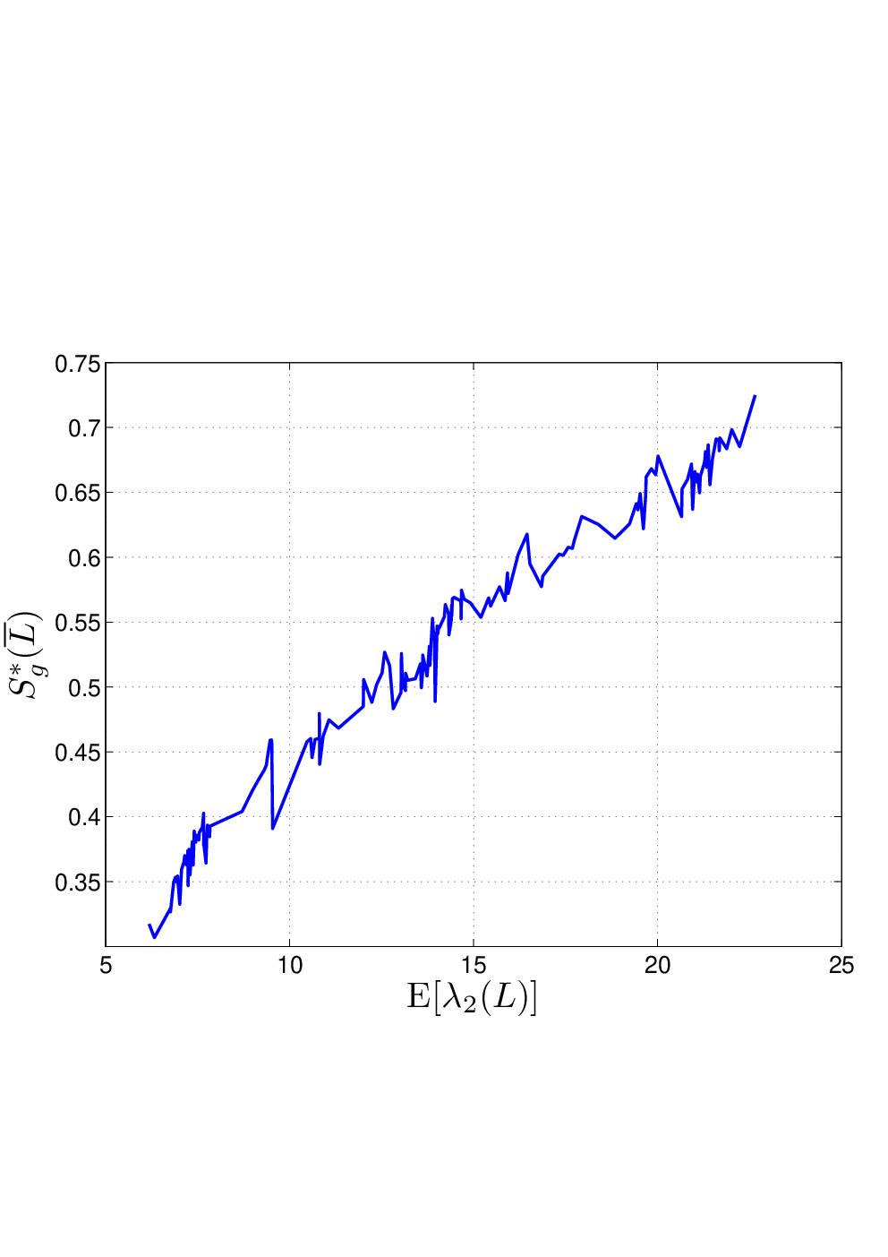
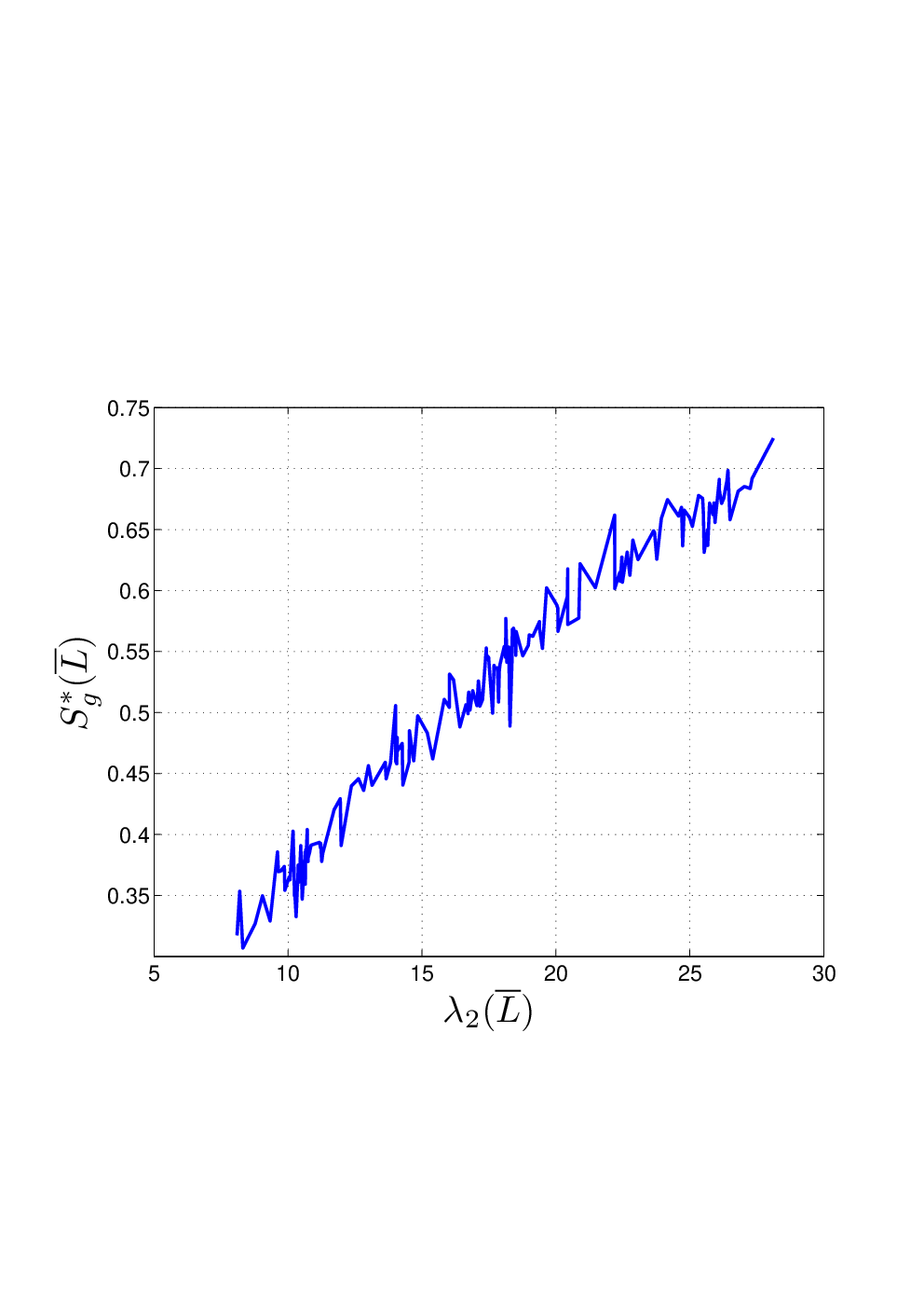
In general, $\widehat{S_{\mbox{\scriptsize{g}}}^{\ast}}\leq S_{\mbox{\scriptsize{g}}}^{\ast}$ . If $S_{\mbox{\scriptsize{g}}}(\alpha,\overline{L})$ was a non-decreasing function of $\lambda_{2}(\overline{L})$ , we would have $\widehat{S_{\mbox{\scriptsize{g}}}^{\ast}}=S_{\mbox{\scriptsize{g}}}^{\ast}$ .

We verify by a numerical study how and in what sense $S_{\mbox{\scriptsize{g}}}^{\ast}\left(\overline{L}\right)$ in (94) increases with $\mbox{E}\left[\lambda_{2}(L)\right]$ and $\lambda_{2}\left(\overline{L}\right)$ . In our simulation, we choose a network with $N=500$ sensors and let the average degree $d_{\mbox{\scriptsize{avg}}}$ of the network vary in steps of $5$ from $10$ to $40$ . For each of these $7$ values of $d_{\mbox{\scriptsize{avg}}}$ , we construct 200 Erdös-Rényi random graphs by choosing at random $M=d_{\mbox{\scriptsize{avg}}}N/2$ edges of the $N(N-1)/2$ possible pairings of vertices in the network. For each of these 200 random graphs, we generate randomly a probability of formation matrix $P$ (hence a probability distribution of $L$ ) by choosing for each edge a weight between $0$ and $1$ from a uniform random distribution. For each such $P$ matrix, we collect statistics on the convergence rate $S_{\mbox{\scriptsize{g}}}^{\ast}\left(\overline{L}\right)$ and $\mbox{E}\left[\lambda_{2}(L)\right]$ by generating $400$ possible $L(i)$ . For each $P$ , we also obtain the corresponding $\lambda_{2}(\overline{L})$ by eqn. (1). This is an extensive and computationally expensive simulation. Fig. 1 displays the results by plotting the convergence rate $S_{\mbox{\scriptsize{g}}}^{\ast}\left(\overline{L}\right)$ with respect to $\mbox{E}\left[\lambda_{2}(L)\right]$ , left plot, and with respect to $\lambda_{2}\left(\overline{L}\right)$ , right plot. These two plots are remarkably similar and both show that, except for local oscillations, the trend of the convergence rate $S_{\mbox{\scriptsize{g}}}^{\ast}\left(\overline{L}\right)$ is to increase with increasing $\mbox{E}\left[\lambda_{2}(L)\right]$ and $\lambda_{2}\left(\overline{L}\right)$ . Of course, $\lambda_{2}\left(\overline{L}\right)$ is much easier to evaluate than $\mbox{E}\left[\lambda_{2}(L)\right]$ . The plots in Fig. 1 confirm that, given a class $\mathcal{D}(U)$ of probability distributions of $L$ , we can set an ordering in $\mathcal{D}(U)$ by evaluating the corresponding $\lambda_{2}\left(\overline{L}\right)$ ’s, in the sense that a larger value of $\lambda_{2}\left(\overline{L}\right)$ leads to a better convergence rate in general (see also [13], where part of these results were presented.) This study shows that optimal topologies with respect to ARCCC should be good topologies with respect to RCCC.

Refer to caption — Fig. 1: Convergence rate $S_{\mbox{\scriptsize{g}}}^{\ast}\left(\overline{L}\right)$ . Left: with varying $\mbox{E}\left[\lambda_{2}(L)\right]$ . Right: with varying $\lambda_{2}\left(\overline{L}\right)$ . The number of vertices is $N=500$ .

VII-B ARCCC: Performance Analysis

To gain insight into ARCCC, we study the dependence of the maximum value of its functional

\phi(U)=\max_{\overline{L}\in\mathcal{D}(U)}\lambda_{2}\left(\overline{L}\right)

(97)

on the value of the communication cost constraint $U$ . We first establish the concavity of $\phi(U)$ .

Lemma 27

Given a cost matrix $C$ , $\phi(U)$ is a concave function of $U$ .

Proof.

Let $0\leq U_{1}\leq U_{2}$ and $0\leq t\leq 1$ . Consider the matrices $\overline{L}^{\ast}_{1}$ and $\overline{L}^{\ast}_{2}$ , such that

\lambda_{2}\left(\overline{L}^{\ast}_{1}\right)=\phi\left(U_{1}\right)\>\>\mbox{and}\>\>\lambda_{2}\left(\overline{L}^{\ast}_{2}\right)=\phi\left(U_{2}\right)

It follows that

\overline{L}^{\ast}_{1}\in\mathcal{D}(U_{1})\>\>\mbox{and}\>\>\overline{L}^{\ast}_{2}\in\mathcal{D}(U_{2})

Let $\overline{L}=t\overline{L}^{\ast}_{1}+(1-t)\overline{L}^{\ast}_{2}$ . Then,

	$\displaystyle-\frac{1}{2}\mbox{Tr}\left\{C\overline{L}\right\}$	$\displaystyle=$	$\displaystyle t\left(-\frac{1}{2}\mbox{Tr}\left\{C\overline{L}^{\ast}_{1}\right\}\right)+(1-t)\left(-\frac{1}{2}\mbox{Tr}\left\{C\overline{L}^{\ast}_{2}\right\}\right)$		(98)
		$\displaystyle\leq$	$\displaystyle tU_{1}+(1-t)U_{2}$		(98)

Hence $\overline{L}\in\mathcal{D}\left(tU_{1}+(1-t)U_{2}\right)$ . From this we conclude that

\phi\left(tU_{1}+(1-t)U_{2}\right)\geq\lambda_{2}\left(\overline{L}\right)

(99)

Now, since $\lambda_{2}\left(\overline{L}\right)$ is a concave function of $\overline{L}$ (see Lemma 4), we get

$\displaystyle\lambda_{2}\left(\overline{L}\right)$	$\displaystyle=$	$\displaystyle\lambda_{2}\left(t\overline{L}^{\ast}_{1}+(1-t)\overline{L}^{\ast}_{2}\right)$	(100)
	$\displaystyle\geq$	$\displaystyle t\lambda_{2}\left(\overline{L}^{\ast}_{1}\right)+(1-t)\lambda_{2}\left(\overline{L}^{\ast}_{2}\right)$
	$\displaystyle=$	$\displaystyle t\phi\left(U_{1})+(1-t)\phi(U_{2}\right)$

Finally, using eqns.(99 and 100), we get

\phi\left(tU_{1}+(1-t)U_{2}\right)\geq t\phi\left(U_{1}\right)+(1-t)\phi\left(U_{2}\right)

(101)

that establishes the concavity of $\phi(U)$ . ∎

We use the concavity of $\phi(U)$ to derive an upperbound on $\phi(U)$ . Recall that $\mathcal{M}$ is the edge set of the complete graph–the set of all possible $N(N-1)/2$ edges. Define the set of realizable edges $\mathcal{E}\subseteq\mathcal{M}$ by

\mathcal{E}\left\{(n,l)\in\mathcal{M}~:~C_{nl}<\infty\right\}

(102)

and by $L_{\mathcal{E}}$ the associated Laplacian. Also, let the total cost $C_{\mbox{\scriptsize{tot}}}$

C_{\mbox{\scriptsize{tot}}}=\sum_{(n,l)~\in~\mathcal{E}}C_{nl}

(103)

The quantity $C_{\mbox{\scriptsize{tot}}}$ is the communication cost per iteration when all the realizable links are used.

Lemma 28

Let $C$ be a cost matrix and $U\geq C_{\mbox{\scriptsize{tot}}}$ . Then $\phi(U)=\lambda_{2}\left(L_{\mathcal{E}}\right)$ . If $\mathcal{E}=\mathcal{M}$ , then $\phi(U)=N$ .

Proof.

The best possible case is when all the network links $(n,l)\in\mathcal{E}$ have probability of formation $P_{nl}=1$ (the links in $\mathcal{E}^{C}$ must have zero probability of formation to satisfy the cost constraint.) In this case, $\overline{L}=L_{\mathcal{E}}$ . Now, if $U\geq C_{\mbox{\scriptsize{tot}}}$ , then $L_{\mathcal{E}}\in\mathcal{D}(U)$ and hence the proof follows. The case $\mathcal{E}=\mathcal{M}$ follows from the fact that, for a complete graph, $\lambda_{2}\left(L_{\mathcal{M}}\right)=N$ (see [19, 20].) ∎

Using the concavity of $\phi(U)$ (Lemma 27), we now derive a performance bound when $U\leq C_{\mbox{\scriptsize{tot}}}$ .

Lemma 29

Let $C$ be a cost matrix. Then

\phi(U)\geq\left(\frac{U}{C_{\mbox{\scriptsize{tot}}}}\right)\lambda_{2}\left(L_{\mathcal{E}}\right),~~0\leq U\leq C_{\mbox{\scriptsize{tot}}}

(104)

If $\mathcal{E}=\mathcal{M}$ , then

\phi(U)\geq\left(\frac{U}{C_{\mbox{\scriptsize{tot}}}}\right)N,~~0\leq U\leq C_{\mbox{\scriptsize{tot}}}

(105)

Proof.

From Lemma 28, $\phi\left(C_{\mbox{\scriptsize{tot}}}\right)\lambda_{2}\left(L_{\mathcal{E}}\right)$ . Then, using the concavity of $\phi(U)$ (see Lemma 27) and the fact that $\phi(0)=0$ , we have, for $0\leq U\leq C_{\mbox{\scriptsize{tot}}}$ ,

$\displaystyle\phi(U)$	$\displaystyle=$	$\displaystyle\phi\left(\left(\frac{U}{C_{\mbox{\scriptsize{tot}}}}\right)C_{\mbox{\scriptsize{tot}}}\right)$	(106)
	$\displaystyle\geq$	$\displaystyle\left(\frac{U}{C_{\mbox{\scriptsize{tot}}}}\right)\phi(C_{\mbox{\scriptsize{tot}}})$
	$\displaystyle=$	$\displaystyle\left(\frac{U}{C_{\mbox{\scriptsize{tot}}}}\right)\lambda_{2}\left(L_{\mathcal{E}}\right)$

This proves the Lemma. The case $\mathcal{E}=\mathcal{M}$ follows easily. ∎

Lemma 28 states what should be expected, namely: to achieve the optimal performance $\lambda_{2}\left(L_{\mathcal{E}}\right)$ one needs no more than $C_{\mbox{\scriptsize{tot}}}$ . Lemma 29 is interesting since it states that the ARCCC optimal topology may achieve better performance than the fraction of communication cost it uses would lead us to expect. The numerical study in the next Section helps to quantify these qualitative assessments.

VII-C Numerical Studies: ARCCC

This Section solves the ARCCC semidefinite programming optimization given by (93). It solves for $P$ , which assigns to each realizable link its probability of error (aka, SNR), or the fraction of time it is expected to be active. We compare the ARCCC optimal topology to a fixed radius connectivity (FRC) topology detailed below. The sensor network is displayed on the left of Fig. 2. We deploy $N=80$ sensors uniformly on a $25\times 25$ square grid on the plane. The set $\mathcal{E}$ of realizable links is constructed by choosing $|\mathcal{E}|=9N$ edges randomly from the set $\mathcal{M}$ of all possible edges. We assume a geometric propagation model: the communication cost is proportional to the square of the Euclidean distance $d_{nl}$ between sensors $n$ and $l$

C_{nl}=\left\{\begin{array}[]{ll}\eta d_{nl}^{2}&\mbox{if $(n,l)\in\mathcal{E}$}\\ \infty&\mbox{otherwise}\end{array}\right.

(107)

where $\eta$ is an appropriately chosen constant. With the FRC network, a sensor $n$ communicates with all other sensors $l$ ( $C_{nl}<\infty$ ) that lie within a radius $R$ . The FRC topology is an instantiation of a fixed, i.e., not random, topology with a fixed cost incurred per iteration.

Fig. 2 on the right plots, as a function of the cost constraint $U$ , the per step convergence gain $S_{\mbox{\scriptsize{g}}}=\widehat{S_{\mbox{\scriptsize{g}}}^{\ast}}$ for the ARCCC optimal topology (top blue line) and the per step convergence gain $S_{\mbox{\scriptsize{g}}}$ of the FRC topology (bottom red line). The ARCCC optimal topology converges much faster than the FRC topology, with the improvement being more significant at medium to lower values of $U$ .

The ARCCC topology has a markedly nonlinear behavior, with two asymptotes: for small $U$ , the sharp increasing asymptote, and the asymptotic horizontal asymptote (when all the realizable edges in $\mathcal{E}$ are used.) The two meet at the knee of the curve $\left(U=6.9\times 10^{4},S_{\mbox{\scriptsize{g}}}=.555\right)$ . For $U=6.9\times 10^{4}$ , the ARCCC convergence rate is $\widehat{S_{\mbox{\scriptsize{g}}}}=.505$ , while FRC’s is $S_{\mbox{\scriptsize{g}}}=.152$ , showing that ARCCC’s topology is $3.3$ times faster than FRC’s. For this example, we compute $C_{\mbox{\scriptsize{tot}}}=14.7\times 10^{4}$ , which shows that ARCCC’s optimal topology achieves the asymptotic performance while using less than 50 % of the communication cost.

VIII Conclusions

The paper presents the design of the topology of a sensor network to maximize the convergence rate of the consensus algorithm as a convex optimization problem. We consider that the communication channels among sensors may fail at random times, that communication among sensors incurs a cost, and that there is an overall communication cost constraint in the network. We first establish necessary and sufficient conditions for mss convergence and a.s. convergence in terms of the expected value of the algebraic connectivity of the random graph defining the network topology and in terms of the algebraic connectivity of the average topology. We apply semidefinite programming to solve numerically for the optimal topology design of the random network subject to the communication cost constraint. Because the topology is random, the solution to this optimization specifies for each realizable link its probability of error (aka, SNR), or the fraction of time the link is expected to be active. We show by a simulation study that the resulting topology design can improve by about 300 % the convergence speed of average consensus over more common designs, e.g., geometric topologies where sensors communicate with sensors within a fixed distance. Our study also shows that the optimal random topology can achieve the convergence speed of a non-random network at a fraction of the cost.

References

[1] J. N. Tsitsiklis, “Problems in decentralized decision making and computation,” Ph.D., Massachusetts Institute of Technology, Cambridge, MA, 1984.
[2] J. N. Tsitsiklis, D. P. Bertsekas, and M. Athans, “Distributed asynchronous deterministic and stochastic gradient optimization algorithms,” IEEE Trans. Autom. Control, vol. AC-31, no. 9, pp. 803–812, september 1986.
[3] A. Jadbabaie, J. Lin, and A. S. Morse, “Coordination of groups of mobile autonomous agents using nearest neighbor rules,” IEEE Trans. Autom. Control, vol. AC-48, no. 6, pp. 988–1001, June 2003.
[4] R. O. Saber and R. M. Murray, “Consensus protocols for networks of dynamic agents,” in 42nd IEEE Conference on Decision and Control, 2003.
[5] L. Xiao, S. Boyd, and S.-J. Kim, “Distributed average consensus with least-mean-square deviation,” 2005, submitted.
[6] V. Blondel, J. Hendrickx, A. Olshevsky, and J. N. Tsitsiklis, “Convergence in multiagent coordiantion, consensus, and flocking,” in ECC-CDC’05, 44th IEEE Conference on Decision and Control and European Control Conference, 2005.
[7] R. Olfati-Saber, “Ultrafast consensus in small-world networks,” in 2005 American Control Conference, vol. 4, June 2005, pp. 2371 – 2378.
[8] S. A. Aldosari and J. M. F. Moura, “Distributed detection in sensor networks: connectivity graph and small-world networks,” in 39th Asilomar Conference on Signals, Systems, and Computers, Pacific Grove, CA, Oct. 2005, pp. 230 – 234.
[9] S. Kar and J. M. F. Moura, “Ramanujan topologies for decision making in sensor networks,” in 44th Allerton Conference on Communication, Control, and Computing, Monticello, IL, Sept. 2006.
[10] ——, “Topology for global average consensus,” in 40th Asilomar Conference on Signals, Systems, and Computers, Pacific Grove, CA, Oct. 2006.
[11] S. Kar, S. A. Aldosari, and J. M. F. Moura, “Topology for distributed inference on graphs,” June 2006, manuscript submitted for publication, 30 pages. [Online]. Available: http://arxiv.org/abs/cs/0606052
[12] R. Olfati-Saber, “Algebraic connectivity ratio of Ramanujan graphs,” Dartmouth College, Thayer School of Engineering, Tech. Rep., 2006, submitted to the 2007 American Control Conference for publication.
[13] S. Kar and J. M. F. Moura, “Distributed average consensus in sensor networks with random link failures,” in The 32nd IEEE International Conference on Acoustics, Speech, and Signal Processing, Honolulu, Hawaii, April 2007.
[14] A. T. Salehi and A. Jadbabaie, “On consensus in random networks,” in The Allerton Conference on Communication, Control, and Computing, Allerton House, IL, September 2007.
[15] S. Boyd, A. Ghosh, B. Prabhakar, and D. Shah, “Randomized gossip algorithms,” IEEE Transactions on Information Theory, vol. 52, pp. 2508 – 2530, June 2006.
[16] R. Olfati-Saber and R. M. Murray, “Consensus problems in networks of agents with switching topology and time-delays,” IEEE Trans. Automat. Contr., vol. 49, no. 9, pp. 1520–1533, Sept. 2004.
[17] Y. Hatano and M. Mesbahi, “Agreement over random networks,” in 43rd IEEE Conference on Decision and Control, vol. 2, Dec. 2004, pp. 2010–2015.
[18] M. Fiedler, “Algebraic connectivity of graphs,” Czechoslovak. Mathematical Journal, vol. 23, no. 98, pp. 298–305, 1973.
[19] F. R. K. Chung, Spectral Graph Theory. Providence, RI : American Mathematical Society, 1997.
[20] B. Mohar, “The Laplacian spectrum of graphs,” in Graph theory, combinatorics, and applications, Y. Alavi, G. Chartrand, O. R. Oellermann, and A. J. Schwenk, Eds. New York: J. Wiley & Sons, 1991, vol. 2, pp. 871–898.
[21] B. Bollobás, Modern Graph Theory. New York, NY: Springer Verlag, 1998.
[22] L. Xiao and S. Boyd, “Fast linear iteration for distributed averaging,” Syst. Contr. Lett., vol. 53, pp. 65–78, Sep. 2004.
[23] S. Camiz and S. Stefani, Matrices and Graphs: Theory and Applications. Singapore: World Scientific Publishing, 1996.
[24] L. Xiao and S. Boyd, “Fast linear iterations for distributed averaging,” Syst. Contr. Lett., vol. 53, pp. 65–78, 2004.
[25] O. Kallenberg, Foundations of Modern Probability, 2nd ed. Springer Series in Statistics., 2002.
[26] G. G. Roussas, An Introduction to Measure-Theoretic Probability. Elsevier Academic Press, Oct. 2004.
[27] J. Galambos, Advanced Probability Theory. New York: Dekker, 1988.
[28] A. Kolmogorov and S. Fomin, Introductory Real Analysis. New York: Dover Publications Inc., 1975.
[29] S. Boyd and L. Vandenberghe, Convex Optimization. New York, NY, USA: Cambridge University Press, 2004.
[30] H. Wolkowicz, R. Saigal, and L. Vandengerghe, Handbook of Semidefinite Programming: Theory, Algorithms, and Applications. Kluwer, 2000.
[31] S. Boyd, “Convex optimization of graph Laplacian eigenvalues,” in International Congress of Mathematicians, vol. 3, 2006, pp. 1311–1319.
[32] Y. Kim and M. Mesbahi, “On maximizing the second smallest eigenvalue of a state-dependent graph Laplacian,” IEEE Transactions on Automatic Control, vol. 51, no. 1, pp. 116 – 120, Jan. 2006.