First of all, we review braided categories and braided Hopf algebras [34, 37]. Braided categories are composed of an object $X$, which is a vector space, a dual object $X^{\ast}$, which is a dual vector space, and morphisms

where $\Bbbk$ is a c-number. The composition of the two morphisms in an obvious way makes the identity. Then the braided categories have also an invertible morphism

where $V,W$ are any pair of vector spaces. Generally the inverse of braiding is not equal to the braiding itself.

The braiding is required to be compatible with the tensor product such that

Then the braiding is also required to be intersectional under any morphisms in a Hopf algebra. For example,

where $Z$ is a vector space.

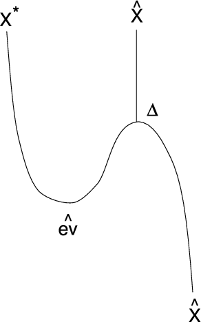
We can represent these axioms in pictorial ways [38]. We write the morphisms, ev, coev, $\psi$, downwards as in Figure 1. Thus the axioms (4) are represented as in Figure 2, and the axioms (5) are represented as in Figure 3.

Next we consider the polynomials of $X$,

where $\mathbf{1}$ is the trivial one-dimensional space. $\widehat{X}$ naturally has the structure of a braided Hopf algebra via

where $\phi\in X$. The tensor product $\otimes$ is the same as the usual product of $X$s, while the new tensor product $\hat{\otimes}$ is the tensor product of $\widehat{X}$s. The coproduct $\Delta$, counit $\epsilon$, antipode $S$ of the products of $X$s are defined inductively by

These axioms are diagrammatically represented in Figure 4.

Next we represent braided quantum field theory [34] in terms of the braided category and the braided Hopf algebra. We take the vector space $X$ as the space of a field $\phi(x)$, where $x$ denotes a general index for independent modes of the field. Thus $\widehat{X}$ is the space of polynomials of the fields such as $\phi(x_{1})\phi(x_{2})\cdots\phi(x_{n})$, and $\mathbf{1}$ correspond to the constant field of unit. We also take the dual vector space $X^{\ast}$ as the space of differentials $\delta/\delta\phi(x)$. We take the evaluation and the coevaluation as follows,

where the distribution and the integration should symbolically be understood, and their detailed forms, which may contain non-trivial measures, depend on each case.

The differential on $\widehat{X}$ is defined by

where

Diagrammatically this is given by Figure 5.

To see whether the map $\mathrm{diff}$ gives really the differential of products, let us compute the differential of $\phi(x)\phi(y)$ as a simple example using the definition (17). This becomes

where we have used the axiom (12) in deriving the third line. If the braiding is trivial, we find that the differential (17) satisfies the usual Leibniz rule.

Generally we find a braided Leibniz rule

and

where $\partial\in X^{\ast}$, $\alpha,\beta\in\widehat{X}$, and we have used a simplified notation

Here $n$ is the degree of $\alpha$, and $[n]_{\psi}$ is called a braided integer defined by

where $\psi_{n,m}$ is a braiding morphism given in Figure 6.

The proofs of the formula (20), (21) are in Appendix A.

Now we define a Gaussian integration, which defines the path integral. The definition is given by

where $w\in\widehat{X}$ is a Gaussian weight. In field theory, $w$ is the exponential of the free part of the action, $e^{-S_{0}}$.

In order to obtain a formula for correlation functions, we define a morphism $\gamma:X^{\ast}\to X$ such that

This morphism is assumed to be commutative with the braiding as in (5). If $w=e^{-S_{0}}$, $\gamma(\partial)=\partial(S_{0})$. In field theory, this is the kinetic part of the action, or the inverse of the propagator.

Starting from (24), we can represent correlation functions of a free field theory in terms of the braided category and the braided Hopf algebra. This is the analog of the Wick theorem in braided quantum field theory. The definition of the free $n$ point correlation function is given by

where the degree of $\alpha$ is $n$. Algebraically, this is given by

where

The proofs of (27), (28), (29) are in Appendix B.

Next we consider correlation functions with the existence of an interaction. For $S=S_{0}+\lambda S_{int}$, a correlation function is perturbatively given by

where $\alpha\in X^{n}$. Introducing a morphism $S_{int}:\Bbbk\to X^{k}$, where $k$ is the degree of $S_{int}$, the correlation function is algebraically given by

Acting $Z_{n}$ on $\alpha\in X^{n}$, we obtain the correlation function (32). One can obviously extend $S_{int}$ to include various interaction terms.

From the results in the preceding subsection, a correlation function can be represented by summation of diagrams obeying the following rules below.

• •

  An $n$-point function $Z_{n}$ is a morphism $X^{n}\to\Bbbk$. Thus a Feynman diagram starts with $n$ strands at the top and must be closed at the bottom.

• •

  The propagator $Z^{(0)}_{2}:X\otimes X\to\Bbbk$ is represented by the left of Figure 7, which is the abbreviation of Figure 9.

• •

  The interaction vertex $S_{int}:\Bbbk\to X^{k}$ is represented by the right of Figure 7. Generally the order of the strands is noncommutative.

• •

  The two kinds of crossings, which are represented in Figure 8, correspond to the braiding and its inverse.

• •

  Any Feynman diagram is built out of propagators, vertices, and crossings, and is closed at the bottom.

We review an action of a general Hopf algebra on vector spaces in a mathematical language [37, 39].

An action $\alpha_{V}$ is a map $\alpha_{V}:\mathcal{A}\otimes V\to V$, where $\mathcal{A}$ is an arbitrary Hopf algebra and $V$ is a vector space (in our case, $\mathcal{A}$ is a symmetry algebra, and $V=X$ or $X^{\ast}$). We will denote the coproduct and the counit of the Hopf algebra²² 2 We omit the antipode. by $\Delta^{\prime}$ and $\epsilon^{\prime}$ to distinguish them from those of the braided Hopf algebra of fields in Section 2. We do not write all the axioms of an action, but our important axioms are the following.

• •

  $\alpha_{V}$ satisfies the following condition.

  $$\alpha_{V}\circ(\cdot\otimes\mathrm{id})=\alpha_{V}\circ(\mathrm{id}\otimes\alpha_{V}),$$

  (34)

  where the equality acts on $\mathcal{A}\otimes\mathcal{A}\otimes V$. This means that $\alpha_{V}((a\cdot b)\otimes V)=\alpha_{V}(a\otimes(\alpha_{V}(b\otimes V)))$, where $a,b\in\mathcal{A}$. In short we can write this as

  $$(a\cdot b)\triangleright V=a\triangleright(b\triangleright V).$$

  (35)

• •

  An action on $\mathbf{1}$, which is in a vector space, is defined by

  $$\alpha_{V}(a\otimes\mathbf{1})=\epsilon^{\prime}(a)\mathbf{1},$$

  (36)

  where $\epsilon^{\prime}(a)$ is the counit of an algebra $a\in\mathcal{A}$.

• •

  An action on a tensor product of vector spaces $V,W$ is defined by

  $$\alpha_{V\otimes W}(a):=((\alpha_{V}\otimes\alpha_{W})\circ\Delta^{\prime})(a)=\sum_{i}\alpha_{V}(a^{i}_{(1)})\otimes\alpha_{W}(a^{i}_{(2)}),~a\in\mathcal{A},$$

  (37)

  where $\Delta^{\prime}(a)=\sum_{i}a^{i}_{(1)}\otimes a^{i}_{(2)}$ is the coproduct of the Hopf algebra $\mathcal{A}$. In the case of a usual Lie-algebraic transformation, its coproduct is given by $\Delta^{\prime}(a)=a\otimes\mathbf{1}+\mathbf{1}\otimes a$, where $\mathbf{1}$ is in $\mathcal{A}$. This gives the usual Leibnitz rule.

• •

  Since a Hopf algebra has the coassociativity that

  $$((\Delta^{\prime}\otimes\mathrm{id})\circ\Delta^{\prime})(a)=((\mathrm{id}\otimes\Delta^{\prime})\circ\Delta^{\prime})(a),$$

  (38)

  the action on a tensor product of vector spaces, which is obtained by the multiple operations of $\Delta^{\prime}$ on $a$, is actually unique. An important consequence is that one can divide the action on a tensor product of vector spaces as

  	$\displaystyle a\triangleright$	$\displaystyle(V_{1}\otimes\cdots\otimes V_{k-1}\otimes V_{k}\otimes\cdots\otimes V_{n})=$
  		$\displaystyle\sum_{i}a_{(1)}^{i}\triangleright(V_{1}\otimes\cdots\otimes V_{k-1})\otimes a_{(2)}^{i}\triangleright(V_{k}\otimes\cdots\otimes V_{n})$		(39)

  for any $k$.

The expression of the correlation functions (33) is perturbative in interactions, but is a full order algebraic description. Therefore we can discuss the symmetry of the theory and the implied relations among correlation functions by using this expression. We may even expect that the relations will hold non-perturbatively.

In usual quantum field theory, if a field theory has a certain symmetry, there is a relation among the correlation functions in the form,

where $\delta_{a}\phi(x)$ is a variation of a field under a transformation $a$, on the assumption that the path integral measure and the action are invariant under the transformation.

If the coproduct of a symmetry algebra is not the usual Lie-algebraic type and thus the Leibniz rule is deformed, the relation will generally have the form,

where $c_{a}^{\cdots}$ are some coefficients. Its essential difference from (40) is the multi-field contributions. In our algebraic language, the relation can be written as

This is equivalent to Figure 10 in our diagrammatic representation. Then we consider what an algebraic structure is required for (42) to hold for any $a$ and $\chi$, i.e. the theory is invariant under the Hopf algebra transformation $\mathcal{A}$.

Let us write the coproduct of an element $a\in\mathcal{A}$ as

where $f^{s},g^{s}\in\mathcal{A}$. Since the coproduct must satisfy the Hopf algebra axiom [37],

$f^{s},g^{s}$ must satisfy

For all the relations among correlation functions to hold, we find the following four conditions for any action $a\in\mathcal{A}$.

• •

  (Condition 1) $S_{int}$ must satisfy

  $$a\triangleright S_{int}=\epsilon^{\prime}(a)S_{int}.$$

  (46)

• •

  (Condition 2) The braiding $\psi$ is an intertwining operator. That is

  $$\psi(a\triangleright(V\otimes W))=a\triangleright\psi(V\otimes W).$$

  (47)

• •

  (Condition 3) $\gamma^{-1}$ and $a$ are commutative,

  $$a\triangleright(\gamma^{-1}(V))=\gamma^{-1}(a\triangleright V).$$

  (48)

• •

  (Condition 4) Under an action $a$, the evaluation map follows

  $$\mathrm{ev}(a\triangleright(X^{\ast}\otimes X))=\epsilon^{\prime}(a)\mathrm{ev}(X^{\ast}\otimes X).$$

  (49)

Condition 1 to 4 are diagrammatically represented in Figure 11. It is clear that, when the algebra $\mathcal{A}$ is generated from a finite number of its independent elements, it is enough for these generators to satisfy these conditions.

Condition 1 is the requirement of the symmetry at the classical level for the interaction. We can extend this condition to

The proof is the following. From a coproduct (43) and its coassociativity (39), the right hand side of (50) is equal to

Since Condition 1 implies

(51) becomes

where we have used (45). Iterating this procedure, we obtain the left-hand side of (50).

Condition 2,3,4 can also be extended to

We can find that these extended conditions (50), (54), (55), (56) can be represented as in Figure 12. In the diagrammatic language, the relation among correlation functions holds if an action can pass downwards through a Feynman diagram and satisfies (36).

In this subsection, we discuss the Poincaré symmetry of the effective noncommutative field theory of three-dimensional quantum gravity coupled with scalar particles, which was obtained in [31] by studying the Ponzano-Regge model [40] coupled with spinless particles. The symmetries of this theory is also known as $\mathrm{DSU}(2)$, which was discussed in [32, 33]. We first review the field theory [10, 31].

Let $\phi(x)$ be a scalar field on a three-dimensional space $x=(x^{1},x^{2},x^{3})$. Its Fourier transformation is given by

where $\kappa$ is a constant, $\mathcal{X}=ix^{i}\sigma_{i}$, and $g=P^{0}-i\kappa P^{i}\sigma_{i}\in\mathrm{SO}(3)$³³ 3 The identification $g\sim-g$ is implicitly assumed. with Pauli matrices $\sigma_{i}$. Here $\int dg$ is the Haar measure of $SO(3)$ and $P^{0}=\pm\sqrt{1-\kappa^{2}P^{i}P_{i}}$ by definition. In the following discussions, we will only deal with the Euclidean case, but the Lorentzian case can also be treated in a similar manner by replacing $\mathrm{SO}(3)$ with $\mathrm{SL}(2,R)$.

The definition of the star product is given by

Differentiating both hands sides of (58) with respect to $P_{1}^{i}:=P^{i}(g_{1})$ and $P_{2}^{j}:=P^{j}(g_{2})$ and then taking the limit $P_{1}^{i},P_{2}^{i}\to 0$, one finds the SO(3) Lie-algebraic space-time noncommutativity [7, 8, 9],

For example, the action⁴⁴ 4 Since in the Ponzano-Regge model the definition of the weight of partition function is $e^{iS}$ despite of Euclidean theory, the sign of the mass term is not the usual one. of a $\phi^{3}$ theory is

where $M^{2}=\frac{\sin^{2}m\kappa}{\kappa^{2}}$. Its momentum representation is

from which it is straightforward to read the Feynman rules.

Some quantum properties of this scalar field theory were analyzed in [10]. As can be seen from (59), the naive translational symmetry is violated. In fact, the violation is rather disastrous. There exists a kind of conserved energy-momentum in the amplitudes of the tree and the planar loop diagrams, but this energy-momentum is not conserved in the non-planar loop diagrams. Moreover, the violation of the energy-momentum conservation does not vanish in the commutative limit $\kappa\rightarrow 0$ due to a mechanism similar to the UV/IR phenomena [11].

In the effective field theory of quantum gravity coupled with spinless particles, however, the Feynman rules contain also a non-trivial braiding rule for each crossing, which comes from a flatness condition in a graph of intersecting particles [31]. This can be incorporated as a braiding between the scalar fields,

in the braided quantum field theory.

From the direct analysis of the Feynman graphs with this braiding rule, one can easily find that the energy-momentum mentioned above is conserved also in the non-planar diagrams. This suggests the existence of a translational symmetry in the quantum field theory. In the sequel, we will discuss the embedding of this field theory into the framework of braided quantum field theory, and will check the four conditions for its translational and rotational symmetries.

We use the momentum representation, and take $X$ as the space of $\tilde{\phi}(g)$ and $X^{\ast}$ as that of $\frac{\delta}{\delta\tilde{\phi}(g)}$. We take the braided Hopf algebra of the fields as follows,

The evaluation and coevaluation maps are given by

From $\gamma(\partial)=\partial S_{0}=(P^{2}(g)-m^{2})\tilde{\phi}(g^{-1})$,

From the algebraic consistencies in Figure 13, the braidings between $X$ and $X^{\ast}$ and the braiding between $X^{\ast}$s are determined to be

In this derivation, we have used the invariance of the Haar measure $d(g^{-1}g^{\prime}g)=dg^{\prime}$.

Now we consider a translational transformation of the field. If we shift $x^{i}$ to $x^{i}+\epsilon^{i}$, a field $\phi(x)$ becomes

Thus in the momentum representation, the translational transformation corresponds to an action

From the requirement that the star product (58) conserve a kind of momentum, the action on a product of fields should be

This determines the coproduct of $P^{i},P^{0}$ as

This coproduct satisfies the coassociativity, which essentially comes from the associativity of the group multiplication.

From the axiom (44), the counit of $P^{i},P^{0}$ is given by

Since the conservation of momentum under the coevaluation map (68) requires that the action of $P^{i}$ on $\int dg(\tilde{\phi}(g)\otimes\frac{\delta}{\delta\tilde{\phi}(g)})$ vanish from (36), the action of $P^{i}$ on $\frac{\delta}{\delta\tilde{\phi}(g)}$ must be

In the following, we see that the momentum algebra satisfies the four conditions (46), (47), (48), (49).

Condition 1 is satisfied since

References

• [1] H. S. Snyder, “Quantized space-time,” Phys. Rev. 71, 38 (1947).
• [2] C. N. Yang, “On Quantized Space-Time,” Phys. Rev. 72, 874 (1947).
• [3] A. Connes and J. Lott, “Particle Models And Noncommutative Geometry (Expanded Version),” Nucl. Phys. Proc. Suppl. 18B, 29 (1991).
• [4] S. Doplicher, K. Fredenhagen and J. E. Roberts, “The Quantum structure of space-time at the Planck scale and quantum fields,” Commun. Math. Phys. 172, 187 (1995) [arXiv:hep-th/0303037].
• [5] N. Seiberg and E. Witten, “String theory and noncommutative geometry,” JHEP 9909, 032 (1999) [arXiv:hep-th/9908142].
• [6] L. J. Garay, “Quantum gravity and minimum length,” Int. J. Mod. Phys. A 10, 145 (1995) [arXiv:gr-qc/9403008].
• [7] N. Sasakura, “Space-time uncertainty relation and Lorentz invariance,” JHEP 0005, 015 (2000) [arXiv:hep-th/0001161].
• [8] J. Madore, S. Schraml, P. Schupp and J. Wess, “Gauge theory on noncommutative spaces,” Eur. Phys. J. C 16, 161 (2000) [arXiv:hep-th/0001203].
• [9] L. Freidel and S. Majid, “Noncommutative harmonic analysis, sampling theory and the Duflo map in 2+1 quantum gravity,” arXiv:hep-th/0601004.
• [10] S. Imai and N. Sasakura, “Scalar field theories in a Lorentz-invariant three-dimensional noncommutative space-time,” JHEP 0009, 032 (2000) [arXiv:hep-th/0005178].
• [11] S. Minwalla, M. Van Raamsdonk and N. Seiberg, “Noncommutative perturbative dynamics,” JHEP 0002, 020 (2000) [arXiv:hep-th/9912072].
• [12] M. Chaichian, P. P. Kulish, K. Nishijima and A. Tureanu, “On a Lorentz-invariant interpretation of noncommutative space-time and its implications on noncommutative QFT,” Phys. Lett. B 604, 98 (2004) [arXiv:hep-th/0408069].
• [13] J. Wess, “Deformed coordinate spaces: Derivatives,” arXiv:hep-th/0408080.
• [14] F. Koch and E. Tsouchnika, “Construction of theta-Poincare algebras and their invariants on M(theta),” Nucl. Phys. B 717, 387 (2005) [arXiv:hep-th/0409012].
• [15] P. Aschieri, C. Blohmann, M. Dimitrijevic, F. Meyer, P. Schupp and J. Wess, “A gravity theory on noncommutative spaces,” Class. Quant. Grav. 22, 3511 (2005) [arXiv:hep-th/0504183].
• [16] P. Aschieri, M. Dimitrijevic, F. Meyer and J. Wess, “Noncommutative geometry and gravity,” Class. Quant. Grav. 23, 1883 (2006) [arXiv:hep-th/0510059].
• [17] X. Calmet and A. Kobakhidze, “Noncommutative general relativity,” Phys. Rev. D 72, 045010 (2005) [arXiv:hep-th/0506157].
• [18] A. Kobakhidze, “Theta-twisted gravity,” arXiv:hep-th/0603132.
• [19] M. Chaichian, P. Presnajder and A. Tureanu, “New concept of relativistic invariance in NC space-time: Twisted Poincare symmetry and its implications,” Phys. Rev. Lett. 94, 151602 (2005) [arXiv:hep-th/0409096].
• [20] M. Chaichian, K. Nishijima and A. Tureanu, “An interpretation of noncommutative field theory in terms of a quantum shift,” Phys. Lett. B 633, 129 (2006) [arXiv:hep-th/0511094].
• [21] A. P. Balachandran, G. Mangano, A. Pinzul and S. Vaidya, “Spin and statistics on the Groenwald-Moyal plane: Pauli-forbidden levels and transitions,” Int. J. Mod. Phys. A 21, 3111 (2006) [arXiv:hep-th/0508002].
• [22] A. P. Balachandran, A. Pinzul and B. A. Qureshi, “UV-IR mixing in non-commutative plane,” Phys. Lett. B 634, 434 (2006) [arXiv:hep-th/0508151].
• [23] F. Lizzi, S. Vaidya and P. Vitale, “Twisted conformal symmetry in noncommutative two-dimensional quantum field theory,” Phys. Rev. D 73, 125020 (2006) [arXiv:hep-th/0601056].
• [24] A. Tureanu, “Twist and spin-statistics relation in noncommutative quantum field theory,” Phys. Lett. B 638, 296 (2006) [arXiv:hep-th/0603219].
• [25] J. Zahn, “Remarks on twisted noncommutative quantum field theory,” Phys. Rev. D 73, 105005 (2006) [arXiv:hep-th/0603231].
• [26] J. G. Bu, H. C. Kim, Y. Lee, C. H. Vac and J. H. Yee, “Noncommutative field theory from twisted Fock space,” Phys. Rev. D 73, 125001 (2006) [arXiv:hep-th/0603251].
• [27] Y. Abe, “Noncommutative quantization for noncommutative field theory,” arXiv:hep-th/0606183.
• [28] A. P. Balachandran, T. R. Govindarajan, G. Mangano, A. Pinzul, B. A. Qureshi and S. Vaidya, “Statistics and UV-IR mixing with twisted Poincare invariance,” Phys. Rev. D 75, 045009 (2007) [arXiv:hep-th/0608179].
• [29] G. Fiore and J. Wess, “On ’full’ twisted Poincare symmetry and QFT on Moyal-Weyl spaces,” arXiv:hep-th/0701078.
• [30] E. Joung and J. Mourad, “QFT with twisted Poincare invariance and the Moyal product,” arXiv:hep-th/0703245.
• [31] L. Freidel and E. R. Livine, “Ponzano-Regge model revisited. III: Feynman diagrams and effective field theory,” Class. Quant. Grav. 23, 2021 (2006) [arXiv:hep-th/0502106].
• [32] K. Noui, “Three dimensional loop quantum gravity: Towards a self-gravitating quantum field theory,” Class. Quant. Grav. 24, 329 (2007) [arXiv:gr-qc/0612145].
• [33] K. Noui, “Three dimensional loop quantum gravity: Particles and the quantum double,” J. Math. Phys. 47, 102501 (2006) [arXiv:gr-qc/0612144].
• [34] R. Oeckl, “Braided quantum field theory,” Commun. Math. Phys. 217, 451 (2001) [arXiv:hep-th/9906225].
• [35] R. Oeckl, “Untwisting noncommutative R**d and the equivalence of quantum field theories,” Nucl. Phys. B 581, 559 (2000) [arXiv:hep-th/0003018].
• [36] L. Freidel, J. Kowalski-Glikman and S. Nowak, “From noncommutative kappa-Minkowski to Minkowski space-time,” arXiv:hep-th/0612170.
• [37] S. Majid, “Foundations of quantum group theory,” Cambridge, UK: Univ. Pr. (1995) 607 p
• [38] S. Majid, “Beyond supersymmetry and quantum symmetry: An Introduction to braided groups and braided matrices,” arXiv:hep-th/9212151.
• [39] A. Klimyk and K. Schmudgen, “Quantum groups and their representations,” Berlin, Germany: Springer (1997) 552 p
• [40] G. Ponzano and T. Regge, in “Spectroscopic and Group Theoretical Methods in Physics” ed. F. Bloch, North-Holland, Amsterdam, (1968).
• [41] L. Alvarez-Gaume, F. Meyer and M. A. Vazquez-Mozo, “Comments on noncommutative gravity,” Nucl. Phys. B 753, 92 (2006) [arXiv:hep-th/0605113].
• [42] A. Agostini, G. Amelino-Camelia, M. Arzano, A. Marciano and R. A. Tacchi, “Generalizing the Noether theorem for Hopf-algebra spacetime symmetries,” arXiv:hep-th/0607221.
• [43] R. J. Szabo, “Quantum field theory on noncommutative spaces,” Phys. Rept. 378, 207 (2003) [arXiv:hep-th/0109162].