Optimal Stimulus and Noise Distributions for Information Transmission via Suprathreshold Stochastic Resonance
Abstract
Suprathreshold stochastic resonance (SSR) is a form of noise enhanced signal transmission that occurs in a parallel array of independently noisy identical threshold nonlinearities, including model neurons. Unlike most forms of stochastic resonance, the output response to suprathreshold random input signals of arbitrary magnitude is improved by the presence of even small amounts of noise. In this paper the information transmission performance of SSR in the limit of a large array size is considered. Using a relationship between Shannon’s mutual information and Fisher information, a sufficient condition for optimality, i.e. channel capacity, is derived. It is shown that capacity is achieved when the signal distribution is Jeffrey’s prior, as formed from the noise distribution, or when the noise distribution depends on the signal distribution via a cosine relationship. These results provide theoretical verification and justification for previous work in both computational neuroscience and electronics.
pacs
02.50.-r,05.40.Ca,89.70.+c,87.19.LaI Introduction
The term ‘stochastic resonance’ describes the situation where a system’s response to some signal is optimized by the presence of random noise, rather than its absence. It occurs in a wide variety of nonlinear physical Gammaitoni et al. 1998 and biological Moss et al. 2004 systems.
In many of the systems and models in which stochastic resonance (SR) has been observed, the essential nonlinearity is a single static threshold, e.g. Wiesenfeld et al. 1994; Bulsara and Zador 1996; Chapeau-Blondeau 1996; Greenwood et al. 1999. It is generally thought that SR cannot occur in such systems for suprathreshold signals, meaning that the amplitude of the input signal needs to be restricted to values smaller than the amplitude of the threshold for SR to occur DeWeese and Bialek 1995.
However, the 1999 discovery of a novel form of SR—known as suprathreshold stochastic resonance (SSR)—showed that this is not always true Stocks 2000. SSR occurs in an array of identical threshold nonlinearities, each of which are subject to independently random additive noise. We refer to this array as the SSR model—see Fig. 1. In this model SR occurs regardless of whether the input signal is entirely subthreshold or not. Furthermore, SSR occurs even for very large input SNRs. This is a further difference to conventional SR, for which the signal is required to be weak compared to the noise.
SSR is a form of aperiodic stochastic resonance Collins et al. 1995; Bulsara and Zador 1996; Morse and Roper 2000 that was first shown to occur by calculating Shannon’s average mutual information for the SSR model Stocks 2000. It was subsequently found that the performance achievable via SSR is maximized when all threshold values are set to the signal mean Stocks 2001a, and that for sufficiently small input SNRs, modifying the thresholds in the model cannot improve information transfer McDonnell et al. 2006.
The SSR model was originally motivated as a model for parallel sensory neurons, such as those synapsing with hair cells in the inner ear Stocks et al. 2002. Although the basic SSR model is non-dynamical, and does not model the many complexities of real neurons, each threshold nonlinearity is equivalent to a Pitts-McCulloch neuron model, and encapsulates the neural coding properties we are interested in—i.e. the generation of action potentials in response to a noisy aperiodic random stimulus. The small input SNRs we focus on are biologically relevant Bialek et al. 1993, particularly so for hair cells, which are subject to substantial Brownian motion Lindner et al. 2005. This leads to much randomness in the release of neurotransmitters at synapses with afferent neurons leading to the cochlear nucleus.
Further justification of the SSR model’s relevance to neural coding is discussed in Hoch et al. 2003; Durrant and Feng 2007; Nikitin et al. 2007, and by extensions of the model to include more biologically realistic neural features. For example, the parallel array has been modified to consist of parallel FitzHugh-Nagumo neuron models Stocks and Mannella 2001, leaky integrate-and-fire neuron models Hoch et al. 2003; Durrant and Feng 2007 and Hodgkin-Huxley models Hoch et al. 2003, and for the case of signal-dependent (multiplicative) noise Nikitin et al. 2007. In all cases the same qualitative results as for the simple threshold model were obtained. The SSR effect has also led to a proposal for improving the performance of cochlear implants for suprathreshold stimuli Stocks et al. 2002, based on the idea that the natural randomness present in functioning cochlear hair cells is missing in patients requiring implants Morse et al. 2007.
The purpose of this paper is to analyze, in a general manner, the information theoretic upper limits of performance of the SSR model. This requires allowing the array size, , to approach infinity. Previous work has discussed the scaling of the mutual information through the SSR model with for specific cases, and found conditions for which the maximum mutual information—i.e. channel capacity—occurs Stocks 2001b; Stocks 2001a; Hoch et al. 2003. In a neural coding context, the question of ‘what is the optimal stimulus distribution?’ for a given noise distribution is discussed numerically for the SSR model in Hoch et al. 2003.
In Sec. II, we significantly extend the results in Stocks 2001b; Stocks 2001a; Hoch et al. 2003, by showing that the mutual information and output entropy can both be written in terms of simple relative entropy expressions—see Eqs. (21) and (22). This leads to a very general sufficient condition, Eq. (25), for achieving capacity in the large regime that can be achieved either by optimizing the signal distribution for a given noise distribution, or optimizing the noise for a given signal. Given the neuroscience motivation for studying the SSR model, this result is potentially highly significant in computational neuroscience, where both optimal stimulus distributions, and optimal tuning curves are often considered Hoch et al. 2003; Brunel and Nadal 1998.
Furthermore, the optimal signal for the special case of uniform noise is shown to be the arcsine distribution (a special case of the Beta distribution), which has a relatively large variance and is bimodal. This result provides theoretical justification for a proposed heuristic method for analog-to-digital conversion based on the SSR model Nguyen 2007. In this method, the input signal is transformed so that it has a large variance and is bimodal.
As a means of verification of our theory, in Sec. III our general results are compared to the specific capacity results contained in Stocks 2001b; Stocks 2001a; Hoch et al. 2003. This leads us to find and justify improvements to these previous results.
Before we proceed however, the remainder of this section outlines our notation, describes the SSR model, and derives some important results that we utilize.
I.1 Information Theoretic Definitions
Recent work using the SSR model has described performance using measures other than mutual information McDonnell et al. 2002a; McDonnell et al. 2002b; Rousseau et al. 2003; Rousseau and Chapeau-Blondeau 2004; McDonnell et al. 2005; Wang and Wu 2005. However, in line with much theoretical neuroscience research Bialek et al. 1993, here we use the information theoretic viewpoint where the SSR model can be considered to be a communications channel Stocks 2000.
Throughout, we denote the probability mass function (PMF) of a discrete random variable, , as , the probability density function (PDF) of a continuous random variable, , as , and the cumulative distribution function (CDF) of as .
All signals are discrete-time memoryless sequences of samples drawn from the same stationary probability distribution. This differs from the detection scenario often considered in SR research, in which the input signal is periodic. Such a signal does not convey new information with an increasing number of samples, and cannot be considered from an information theoretic viewpoint DeWeese and Bialek 1995.
Consider two continuous random variables, and , with PDFs and , with the same support, . The relative entropy—or Kullback-Liebler divergence—between the two distributions is defined as Cover and Thomas 1991
| (1) |
Suppose and have joint PDF, . Shannon’s mutual information between and is defined as the relative entropy between the joint PDF and the product of the marginal PDFs Cover and Thomas 1991,
| (2) |
where is the entropy of and is the average conditional entropy of given .
The definition of mutual information also holds for discrete random variables, and for one variable discrete and one continuous. The entropy of a discrete random variable, , is given by
| (3) |
while a continuous random variable, , has differential entropy
| (4) |
In this paper we are interested in the case of continuous with support and discrete, with states, in which case the average conditional entropy of given is
| (5) |
In information theory, the term channel capacity is defined as being the maximum achievable mutual information of a given channel Cover and Thomas 1991. Suppose is the source random variable, and is the random variable at the output of the channel. Usually, the channel is assumed to be fixed and the maximization performed over all possible source PDFs, . The channel capacity, , can be expressed as the optimization problem,
| (6) |
Usually there are prescribed constraints on the source distribution such as a fixed average power, or a finite alphabet Cover and Thomas 1991. In Sec. III we will also consider the more stringent constraint that the PDF of the source is known other than its variance. In this situation, channel capacity is determined by finding the optimal source variance, or as is often carried out in SR research, the optimal noise variance.
I.2 SSR Model
Fig. 1 shows a schematic diagram of the SSR model. The array consists of parallel threshold nonlinearities—or ‘devices’, each of which receive the same random input signal, , with PDF . The –th device in the model is subject to continuously valued iid—independent and identically distributed—additive random noise, (), with PDF . Each noise signal is required to also be independent of the signal, . The output of each device, , is unity if the input signal, , plus the noise on that device’s threshold, , is greater than the threshold value, . The output signal is zero otherwise. The outputs from each device, , are summed to give the overall output signal, . This output is integer valued, , and is therefore a quantization (digitization) of McDonnell et al. 2005.
The conditional PMF of the output given the input is . We abbreviate this to . The output distribution is
| (7) |
The mutual information between and is that of a semi-continuous channel Stocks 2000, and can be written as
| (8) |
To progress further we use the notation introduced in Stocks 2000. Let be the probability of the –th threshold device giving output in response to input signal value, . If the noise CDF is , then
| (9) |
As noted in Stocks 2000, is given by the binomial distribution as
| (10) |
and Eq. (I.2) reduces to
| (11) |
Numerically evaluating Eq. (I.2) as a function of input SNR for given signal and noise distributions finds that the mutual information has a unimodal stochastic resonance curve for , even when the signal and noise are both suprathreshold—i.e. the threshold value, , is set to the signal mean Stocks 2001a; McDonnell et al. 2002a.
Further analytical simplification of Eq. (I.2) is possible in the case where the signal and noise PDFs are identical with the same variance, i.e. Stocks 2001a. The result is
| (12) |
What is quite remarkable about this result is that the mutual information is independent of the shape of the PDFs of the signal and noise, other than that . This means that both PDFs have the same shape, but may possibly have different means, and be mutually reversed along the -axis about their means. In Sec. II.4 we compare the mutual information of Eq. (12) with our calculations of the general channel capacity.
I.3 Describing SSR Using a Single PDF,
We now show that the mutual information in the SSR model depends solely on , and an auxiliary PDF, . This PDF is shown to be that of the random variable describing the conditional average output of the SSR model, given that the input signal is .
I.3.1 as the PDF of the Average Transfer Function
Although the output of the SSR model, , is a discrete random variable, the conditional expected value of , given the input is , is a continuous random variable, since is. We label this random variable as . Since the PMF of given is the binomial PMF as in Eq. (10), we know that is the random variable that results from . Inverting this gives .
The PDF of can be derived from , since provides an invertible transformation of , with PDF , to , with PDF . Using the well known expression for the resultant PDF, and provided the support of is contained in the support of —since otherwise does not necessarily exist—we have
| (13) |
Our condition regarding the supports of the signal and noise ensures that . If we make a further change to a new random variable, , via , the PDF of is
| (14) |
and the PDF of can be written as
| (15) |
which illustrates the physical significance of the auxiliary PDF, , as the PDF of .
I.3.2 Mutual Information in Terms of
I.3.3 Entropy of the random variable,
If we make a change of variable from to , and note that , the entropy of can be written as
| (18) |
which is the negative of the relative entropy between the signal PDF, and the noise PDF reversed about and shifted by . In the event that the noise PDF is an even function about its mean, and is equal to the signal mean, then the entropy of is simply the negative of the relative entropy between the signal and noise PDFs.
I.3.4 Examples of the PDF
The PDF can be derived for specific signal and noise distributions. Table 1 lists for several cases where the signal and noise share the same distribution and a mean of zero, but with not necessarily equal variances. The threshold value, , is also set to zero.
For each case considered, the standard deviation of the noise can be written as , where is a positive constant, and the standard deviation of the signal can be written . We find that in each case is a function of a single parameter that we call the noise intensity, . Given this, from Eq. (I.3.2), it is clear that the mutual information must be a function only of the ratio, , so that it is invariant to a change in provided changes by the same proportion. This fact is noted to be true for the Gaussian case in Stocks 2000, and the uniform case in Stocks 2001a, but here we have illustrated why.
We note however, that if is not equal to the signal mean, then will depend on the ratio , as well as and , and therefore so will the mutual information.
Table 1 also lists the entropy of for three cases where an analytical expression could be found.
I.4 Large SSR: Literature Review and Outline of This Paper
In the absence of noise, the maximum mutual information is the maximum entropy of the output signal, . It has been shown for very specific signal and noise distributions that the mutual information in the SSR model scales with for large Stocks 2001b; Stocks 2001a. This means that the channel capacity for large under the specified conditions is about half the maximum noiseless channel capacity. This situation is discussed in Sec. III.
The only other work to consider SSR in the large regime finds that the optimal noise intensity for Gaussian signal and noise occurs for Hoch et al. 2003. Unlike Stocks 2001b—which uses the exact expression of Eq. (12), and derives a large expression by approximating the summation with an integral—Hoch et al. 2003 begins by using a Fisher information based approximation to the mutual information.
In Appendix A.1 we re-derive the formula of Hoch et al. 2003 in a different manner, which results in new large approximations for the output entropy, as well as the mutual information. These approximations provide the basis for the central result of this paper, which is a general sufficient condition for achieving channel capacity in the SSR model, for any arbitrary specified signal or noise distribution. This is discussed in Section II. These new general results are compared with the specific results of Stocks 2001b; Stocks 2001a; Hoch et al. 2003 in Sec. III.
II A General Expression for the SSR Channel Capacity for Large
Fisher information Lehmann and Casella 1998; Cover and Thomas 1991 has previously been discussed in numerous papers on both neural coding Bethge et al. 2002 and stochastic resonance Greenwood et al. 2004, and both Stemmler 1996; Greenwood et al. 2000. However, most SR studies using Fisher information consider only the case where the signal itself is not a random variable. When it is a random variable, it is possible to connect Fisher information and Shannon mutual information under special conditions, as discussed in Stemmler 1996; Brunel and Nadal 1998; Kang and Sompolinsky 2001; Hoch et al. 2003.
It is demonstrated in Hoch et al. 2003 that the Fisher information at the output of the SSR model as a function of input signal value , is given by
| (19) |
In Hoch et al. 2003, Eq. (19) is used to approximate the large mutual information in the SSR model via the formula
| (20) |
This expression—which is derived under much more general circumstance in Clarke and Barron 1990; Brunel and Nadal 1998—relies on an assumption that an efficient Gaussian estimator for can be found from the output of the channel, in the limit of large .
In Appendix A.1 we outline an alternative derivation to Eq. (20)—from which Eq. (19) can be inferred—that is specific to the SSR model, and provides additional justification for its large asymptotic validity. This alternative derivation allows us to find individual expressions for both the output entropy and conditional output entropy. This derivation makes use of the auxiliary PDF, , derived in Sec. I.3. The significance of this approach is that it leads to our demonstration of the new results that the output entropy can be written for large as
| (21) |
while the mutual information can be written as
| (22) |
where is a PDF known as Jeffrey’s prior,
| (23) |
It is proven in Appendix A.2 that for the SSR model Eq. (23) is indeed a PDF. This is a remarkable result, as in general Jeffrey’s prior has no such simple form. Substitution of Eq. (23) into Eq. (22) and simplifying leads to Eq. (20), which verifies this result.
By inspection of Eq. (19), can be derived from knowledge of the noise PDF, , since
| (24) |
II.1 A Sufficient Condition for Optimality
Since relative entropy is always non-negative, from Eq. (22) a sufficient condition for achieving the large channel capacity is that
| (25) |
with the resultant capacity as
| (26) |
Eq. (26) holds provided the conditions for the approximation given by Eq. (20) hold. Otherwise, the RHSs of Eqs. (21) and (22) give lower bounds. This means that for the situations considered previously in Hoch et al. 2003; Stocks 2001b where the signal and noise both have the same distribution (but different variances), we can expect to find channel capacity that is less than or equal to that of Eq. (26). This is discussed in Sec. III.
The derived sufficient condition of Eq. (25) leads to two ways in which capacity can be achieved, (i) an optimal signal PDF for a given noise PDF, and (ii) an optimal noise PDF for a given signal PDF.
II.2 Optimizing the Signal Distribution
Assuming Eq. (20) holds, the channel capacity achieving input PDF, , can be found for any given noise PDF from Eqs. (24) and (25) as
| (27) |
II.2.1 Example: Uniform Noise
Suppose the iid noise at the input to each threshold device in the SSR model is uniformly distributed on the interval so that it has PDF
| (28) |
Substituting Eq. (28) and its associated CDF into Eq. (27), we find that the optimal signal PDF is
| (29) |
This PDF is in fact the PDF of a sine-wave with uniformly random phase, amplitude , and mean . A change of variable to the interval via the substitution results in the PDF of the Beta distribution with parameters and , also known as the arcsine distribution. As mentioned in Sec. I, this result provides some theoretical justification for the analog-to-digital conversion method proposed in Nguyen 2007.
This Beta distribution is bimodal, with the most probable values of the signal those near zero and unity. Similar results for an optimal input distribution in an information theoretic optimization of a neural system have been found in Schreiber et al. 2002. These results were achieved numerically using the Blahut-Arimoto algorithm often used in information theory to find channel capacity achieving source distributions, or rate-distortion functions Cover and Thomas 1991.
II.2.2 Gaussian Noise
Suppose the iid noise at the input to each threshold device has a zero mean Gaussian distribution with variance , with PDF
| (30) |
Substituting Eq. (30) and its associated CDF into Eq. (27), gives the optimal signal PDF. The resultant expression for does not simplify much, and contains the standard error function, Spiegel and Liu 1999.
We are able to verify that the resultant PDF has the correct shape via Fig. 8 in Hoch et al. 2003, which presents the result of numerically optimizing the signal PDF, , for unity variance zero mean Gaussian noise, , and . As with the work in Schreiber et al. 2002, the numerical optimization is achieved using the Blahut-Arimoto algorithm. It is remarked in Hoch et al. 2003 that the optimal is close to being Gaussian. This is illustrated by plotting both and a Gaussian PDF with nearly the same peak value as . It is straightforward to show that a Gaussian with the same peak value as our analytical has variance . If the signal was indeed Gaussian, then we would have , which is very close to the value calculated for actual Gaussian signal and noise in Sec. III.
Our analytical from Eqs. (30) and (27), with , is plotted on the interval in Fig. 2, along with a Gaussian PDF with variance . Clearly the optimal signal PDF is very close to the Gaussian PDF. Our Fig. 2 is virtually identical to Fig. 8 in Hoch et al. 2003. It is emphasized that the results in Hoch et al. 2003 were obtained using an entirely different method that involves numerical iterations, and therefore provides excellent validation of our theoretical results.
II.3 Optimizing the Noise Distribution
We now assume that the signal distribution is known and fixed. We wish to achieve channel capacity by finding the optimal noise distribution. It is easy to show by integrating Eq. (24) that the CDF corresponding to the PDF, , evaluated at , can be written in terms of the CDF of the noise distribution as
| (31) |
If we now let , then , and rearranging Eq. (31) gives the optimal noise CDF in terms of the signal CDF as
| (32) |
Differentiating gives the optimal noise PDF as a function of the signal PDF and CDF,
| (33) |
Unlike optimizing the signal distribution, which is the standard way for achieving channel capacity in information theory Cover and Thomas 1991, we have assumed a signal distribution, and found the ‘best’ noise distribution, which is equivalent to optimizing the channel, rather than the signal.
II.3.1 Example: Uniform Signal
Suppose the signal is uniformly distributed on the interval . From Eqs. (32) and (33), the capacity achieving noise distribution has CDF
| (34) |
and PDF
| (35) |
Substitution of and into Eq. (19) finds the interesting result that the Fisher information is constant for all ,
| (36) |
This is verified in Eq. (37) below.
II.4 Consequences of Optimizing the Large Channel Capacity
II.4.1 Optimal Fisher Information
Regardless of whether we optimize the signal for given noise, or optimize the noise for a given signal, it is straightforward to show that the Fisher information can be written as a function of the signal PDF,
| (37) |
Therefore, the Fisher information at large channel capacity is constant for the support of the signal iff the signal is uniformly distributed. The optimality of constant Fisher information in a neural coding context is studied in Bethge et al. 2002.
II.4.2 The Optimal PDF
A further consequence that holds in both cases is that the ratio of the signal PDF to the noise PDF is
| (38) |
This is not a PDF. However, if we make a change of variable via we get the PDF discussed in Sec. I.3, which for channel capacity is
| (39) |
This optimal is in fact the PDF of the beta distribution with parameters and , i.e. the arcsine distribution. It is emphasised that this result holds regardless of whether the signal PDF is optimised for a given noise PDF or vice versa.
II.4.3 Output Entropy at Channel Capacity
II.4.4 The Optimal Output PMF is Beta-Binomial
Suppose we have signal and noise such that —i.e. the signal and noise satisfy the sufficient condition, Eq. (25)—but that is not necessarily large. We can derive the output PMF for this situation, by substituting Eq. (39) into Eq. (17) to get
| (42) |
where is a Beta function. This PMF can be recognized as that of the Beta-binomial—or negative hypergeometric—distribution with parameters , Evans et al. 2000. It is emphasized that Eq. (II.4.4) holds as an exact analytical result for any .
II.4.5 Analytical Expression for the Mutual Information
The exact expression for the output PMF of Eq. (II.4.4) allows exact calculation of both the output entropy, and the mutual information without need for numerical integration, using Eq. (I.3.2). This is because when , the integrals in Eq. (I.3.2) can be evaluated exactly to get
| (43) |
The exact values of and the corresponding output entropy, , are plotted in Fig. 3(a) for . For comparison, the exact of Eq. (12), which holds for , is also plotted, as well as the corresponding entropy, . It is clear that is always larger than the mutual information of the case, and that is always less than its entropy, which is the maximum output entropy.
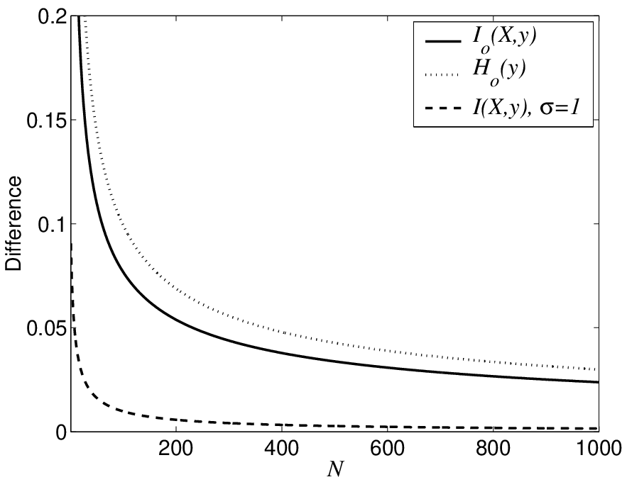
To illustrate that the large expressions derived are lower bounds to the exact formula plotted in Fig. 3(a), and that the error between them decreases with , Fig. 3(b) shows the difference between the exact and the large mutual information and output entropy. This difference clearly decreases with increasing .
II.5 A Note on the Output Entropy
The SSR model has been described in terms of signal quantization theory in McDonnell et al. 2005, and compared with the related process of companding in Amblard et al. 2006. In this context quantization means the conversion of a continuously valued signal to a discretely valued signal that has only a finite number of possible values. Quantization in this sense occurs in analog-to-digital converter circuits, lossy compression algorithms, and in histogram formation Gersho and Gray 1992. For a deterministic scalar quantizer with output states, threshold values are required. In quantization theory, there is a concept of high resolution quantizers, in which the distribution of threshold values can be described by a point density function, . For such quantizers, it can be shown that the quantizer output, , in response to a random variable, , has entropy Gersho and Gray 1992. This is strikingly similar to our Eq. (21) for the large output entropy of the SSR model. In fact, since the noise that perturbs the fixed threshold value, , is additive, each threshold acts as an iid random variable with PDF , and therefore for large , acts as a density function describing the relative frequency of threshold values as a function of , just as does for a high resolution deterministic quantizer.
For deterministic quantizers, the point density function can be used to approximate the high resolution distortion incurred by the quantization process. For the SSR model however, since the quantization has a random aspect, the distortion has a component due to randomness as well as lossy compression, and cannot be simply calculated from . Instead, one can use the Fisher information to calculate the asymptotic mean square error distortion, which is not possible for deterministic high resolution quantizers.
III Channel Capacity for Large and ‘Matched’ Signal and Noise
Unlike the previous section, we now consider channel capacity under the constraint of ‘matched’ signal and noise distributions—i.e. where both the signal and noise, while still independent, have the same distribution, other than their variances. The mean of both signal and noise is zero and the threshold value is also . In this situation the mutual information depends solely on the ratio , which is the only free variable. Finding channel capacity is therefore equivalent to finding the optimal value of noise intensity, . Such an analysis provides verification of the more general capacity expression of Eq. (26), which cannot be exceeded.
Furthermore, inspection of Eq. (65) shows that the large approximation to the mutual information consists of a term that depends on and a term that depends only on . This shows that for large the channel capacity occurs for the same value of —which we denote as —for all .
This fact is recognized in both Stocks 2001b for uniform signal and noise—where —and Hoch et al. 2003, for Gaussian signal and noise. Here, we investigate the value of and the mutual information at for other signal and noise distributions, and compare the channel capacity obtained with the case where . This comparison finds that the results of Hoch et al. 2003 overstates the true capacity, and that large results in Stocks 2001b; Stocks 2001a need to be improved to be consistent with the central results of this paper.
From Eq. (22), channel capacity for large occurs for the value of that minimizes the relative entropy between and . If we let
| (44) |
then from Eq. (20), it is also clear that this minimization is equivalent to solving the following problem,
| (45) |
This is exactly the formulation stated in Hoch et al. 2003. Problem (45) can be equivalently expressed as
| (46) |
where we have assumed that both the signal and noise PDFs are even functions. The function can be found for any specified signal and noise distribution by numerical integration, and Problem (46) easily solved numerically. If an exact expression for the relative entropy term is known, then only needs to be numerically calculated.
Table 2 gives the result of numerically calculating the value of , and the corresponding large channel capacity, , for a number of distributions. In each case, , as required by Eq. (26). The difference between capacity and is about bits per sample. In the limit of large , this shows that capacity is almost identical, regardless of the distribution. However, the value of at which this capacity occurs is different in each case.
As discussed in Sec. I.2, the mutual information is identical whenever the signal and noise PDFs are identical, i.e. . It is shown below in Eq. (48) that for large the mutual information at is . Given that the channel capacity is slightly larger than this, as indicated by Table 2, for each case there is a constant difference between the channel capacity and the mutual information at . This value is also listed in Table 2.
III.1 Improvements to Previous Large Approximations
We now use the results of Sec. II to show that previous large expressions for the mutual information in the literature for the , Gaussian and uniform cases can be improved.
III.1.1 SSR for Large and
We now consider the situation where , so that . It is shown in Stocks 2001a that in this case as approaches infinity, Eq. (12) reduces to
| (47) |
To show that this expression can be improved, we begin with the version of Eq. (20) given by Eq. (65). When we have and . The integrals in Eq. (65) can be solved to give the large mutual information at as
| (48) |
Although Eqs. (47) and (48) agree as , the constant terms do not agree. It is shown in Appendix A.3 that the discrepancy can be resolved by improving on the approximation to the average conditional entropy, , made in Stocks 2001a. The output entropy at can be shown to be simply Stocks 2001a. Subtracting Eq. (A.3) from and letting approach infinity gives
| (49) |
which does have a constant term which agrees with Eq. (48). The explanation of the discrepancy is that Stocks 2001a uses the Euler-Maclaurin summation formula to implicitly calculate in the large approximation to . Using Stirling’s approximation for , as done here, gives a more accurate approximation.
The increased accuracy of Eq. (48) can be verified by numerically comparing both Eq. (48) and Eq. (47) with the exact expression for of Eq. (12), as increases. The error between the exact expression and Eq. (48) approaches zero as increases, whereas the error between Eq. (12) and Eq. (47) approaches a nonzero constant for large of bits per sample.
III.1.2 Uniform Signal and Noise
A derivation is given in Stocks 2001b of an exact expression for for uniform signal and noise and . In addition, Stocks 2001b finds a large approximation to the mutual information. Using the same arguments as for the case, this approximation can be improved to
| (50) |
The accuracy of Eq. (50) can be verified by numerical comparison with the exact formula in Stocks 2001b, as increases. If one replicates Fig. 3 of Stocks 2001b in this manner, it is clear that Eq. (50) is the more accurate approximation.
Differentiating Eq. (50) with respect to and setting to zero obtains the optimal value of as
| (51) |
The channel capacity at is
| (52) |
Clearly, , and the capacity approaches , which agrees with Eq. (49). Expressions for and the corresponding capacity for large are also given in Stocks 2001b. Again, these are slightly different to Eqs. (51) and (52), due to the slightly inaccurate terms in the large approximation to . However the important qualitative result remains the same, which is that the channel capacity scales with and the value of which achieves this asymptotically approaches unity.
III.1.3 Gaussian Signal and Noise
In Hoch et al. 2003, an analytical approximation for for the specific case of Gaussian signal and noise is derived using a Taylor expansion of the Fisher information inside the integral in Eq. (20). We give a slightly different derivation of this approach that uses the PDF .
We begin with Problem (46). Solving this problem requires differentiating with respect to and solving for zero. From Table 1, the derivative of the relative entropy between and is
| (53) |
For the second term, , we take the lead from Hoch et al. 2003 and approximate by its second order Taylor series expansion Spiegel and Liu 1999. The result is that
| (54) |
Numerical testing finds that the approximation of Eq. (54) appears to be quite accurate for all , as the relative error is no more than about percent for . However, as we will see, this is inaccurate enough to cause the end result for the approximate channel capacity to significantly overstate the true channel capacity.
Taking the derivative of Eq. (54) with respect to , subtracting it from Eq. (53), setting the result to zero and solving for gives the optimal value of found in Hoch et al. 2003, .
An expression for the mutual information at can be found by back-substitution. Carrying this out gives the large channel capacity for Gaussian signal and noise as
| (55) |
which can be written as .
Although Eq. (55) is close to correct, recall from Sec. II that capacity must be less than and hence Eq. (55) significantly overstates the true capacity.
Acknowledgements.
This work was funded by the Australian Research Council, an Australian Academy of Science Young Researcher’s Award, as well as EPSRC grant EP/C523334/1, and we gratefully acknowledge this support. The authors would also like to thank Priscilla Greenwood, of Arizona State University, Pierre-Olivier Amblard of Laboratoire des Images et des Signaux, France, Thinh Nguyen of Oregon State University and Simon Durrant of the University of Plymouth, UK, for valuable discussions and generous provision of preprints, and the anonymous referees, whose comments have led to significant improvements in this paper.Appendix A Derivations
A.1 Mutual Information for Large and Arbitrary
This appendix contains derivations of the large approximations to the output entropy and mutual information discussed in Sec. II.
A.1.1 Conditional Output Entropy
An approximation to the conditional output entropy, , can be derived by noting that for large the binomial distribution can be approximated by a Gaussian distribution with the same mean and variance—i.e. and respectively. Provided we have
| (56) |
The average conditional output entropy is , where
| (57) |
Using the well known result for the entropy of a Gaussian random variable Cover and Thomas 1991 we can write
| (58) |
Multiplying both sides of Eq. (58) by and integrating over all gives
| (59) |
Eq. (A.1.1) can be verified for the case where , since this means and . Consequently Eq. (A.1.1) reduces to which agrees precisely with Eq. (74). This approximation breaks down when is close to zero or unity. Furthermore, Eq. (A.1.1) holds exactly only for values of for which is exactly Gaussian. Otherwise, is strictly less than the approximation given.
A.1.2 Output Distribution and entropy
For large , since is Gaussian, approaches a delta function located at . From Eqs. (7) and (17), this means that can be written in terms of the PDF of the average transfer function, , as
| (60) |
This result can be derived more rigorously using saddlepoint methods Brunel and Nadal 1998.
Consider the case where the signal and noise both have the same distribution but different variances. When the noise intensity, , then , whereas for , we have . From Eq. (60), this means and are either zero or infinite. However, for finite , there is some finite nonzero probability that all output states are on or off. Indeed, at , we know that , and at , . Furthermore, for finite , Eq. (60) does not guarantee that . To increase the accuracy of our approximation by ensuring and are always finite, and that forms a valid PMF, we define a new approximation as
| (61) |
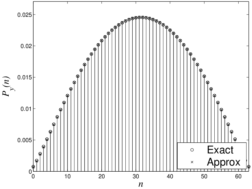
Fig. 4 shows that the approximation given by is highly accurate for as small as , for both smaller and larger than unity.
Consider the entropy of the discrete random variable . Making use of Eq. (60), we have
| (62) |
Suppose that the summations above can be approximated by integrals, without any remainder terms. Carrying this out and then making the change of variable gives
| (63) |
where is the differential entropy of the random variable . Performing a change of variable in Eq. (A.1.2) of gives
| (64) |
This result shows that for large is approximately the sum of the number of output bits and the negative of the relative entropy between and . Therefore, since relative entropy is always non-negative, the approximation to given by Eq. (64) is always less than or equal to . This agrees with the known expression for in the specific case of of , which holds for any .
A.1.3 Mutual Information
Subtracting Eq. (A.1.1) from Eq. (A.1.2) gives a large approximation to the mutual information as
| (65) |
As discussed in the main text, the mutual information scales with . The importance of the -independent terms in Eq. (65) is that they determine how the mutual information varies from for different PDFs, .
Fig. 5 shows, as examples, the approximation of Eq. (65), as well as the exact mutual information—calculated by numerical integration—for the Gaussian and Laplacian cases, for a range of and increasing . As with the output entropy, the mutual information approximation is quite good for , but worsens for smaller . However, as increases the approximation improves.
Eq. (65) can be rewritten via the change of variable, , as
| (66) |
Rearranging Eq. (A.1.3) gives Eq. (20)—with the Fisher information, , given by Eq. (19)—which is precisely the same as that derived in Hoch et al. 2003 as an asymptotic large expression for the mutual information. Our analysis extends Hoch et al. 2003 by finding large approximations to both and , as well as the output distribution, . We have also illustrated the role of the PDF, , in these approximations, and justified the use of Eq. (20) for the SSR model.
A.2 Proof that is a PDF
As shown in Hoch et al. 2003, the Fisher information for the SSR model is given by Eq. (19). Consider as in Eq. (24). Since is a PDF and is the CDF of evaluated at , we have . Letting , Eq. (24) can be written as
| (67) |
Suppose has support . Integrating over all gives
| (68) |
which means is a PDF.
A.3 for large and
Here we derive a large approximation to used in Sec. III.1.1. For the output PMF is Stocks 2001a. Using this, it can be shown that
| (69) |
We will now see that both terms of Eq. (69) can be simplified by approximations that hold for large . Firstly, for the term, we can make use of Stirling’s formula Spiegel and Liu 1999, which is valid for large ,
| (70) |
This approximation is particularly accurate if the log is taken of both sides, which we require. Secondly, the sum in the second term of Eq. (69) can be approximated by an integral and simplified by way of the Euler-Maclaurin summation formula Spiegel and Liu 1999. The result is
| (71) |
Subtracting Eq. (71) from the log of Eq. (70) gives
| (72) |
where we have used . When Eq. (A.3) is substituted into an exact expression for given in Stocks 2001a, we get
| (73) |
The final result is that for large ,
| (74) |
References
- Gammaitoni et al. (1998) L. Gammaitoni, P. Hänggi, P. Jung, and F. Marchesoni, Reviews of Modern Physics 70, 223 (1998).
- Moss et al. (2004) F. Moss, L. M. Ward, and W. G. Sannita, Clinical Neurophysiology 115, 267 (2004).
- Wiesenfeld et al. (1994) K. Wiesenfeld, D. Pierson, E. Pantazelou, C. Dames, and F. Moss, Phys. Rev. Lett. 72, 2125 (1994).
- Bulsara and Zador (1996) A. R. Bulsara and A. Zador, Phys. Rev. E 54, R2185 (1996).
- Chapeau-Blondeau (1996) F. Chapeau-Blondeau, Phys. Rev. E 53, 5469 (1996).
- Greenwood et al. (1999) P. E. Greenwood, L. M. Ward, and W. Wefelmeyer, Phys. Rev. E 60, 4687 (1999).
- DeWeese and Bialek (1995) M. DeWeese and W. Bialek, Nuovo Cimento 17, 733 (1995).
- Stocks (2000) N. G. Stocks, Phys. Rev. Lett. 84, 2310 (2000).
- Collins et al. (1995) J. J. Collins, C. C. Chow, and T. T. Imhoff, Phys. Rev. E 52, R3321 (1995).
- Morse and Roper (2000) R. P. Morse and P. Roper, Phys. Rev. E 61, 5683 (2000).
- Stocks (2001a) N. G. Stocks, Phys. Rev. E 63, 041114 (2001a).
- McDonnell et al. (2006) M. D. McDonnell, N. G. Stocks, C. E. M. Pearce, and D. Abbott, Phys. Lett. A 352, 183 (2006).
- Stocks et al. (2002) N. G. Stocks, D. Allingham, and R. P. Morse, Fluct. Noise Lett. 2, L169 (2002).
- Bialek et al. (1993) W. Bialek, M. DeWeese, F. Rieke, and D. Warland, Physica A 200, 581 (1993).
- Lindner et al. (2005) J. F. Lindner, M. Bennett, and K. Wiesenfeld, Phys. Rev. E 72, 051911 (2005).
- Hoch et al. (2003) T. Hoch, G. Wenning, and K. Obermayer, Phys. Rev. E 68, 011911 (2003).
- Durrant and Feng (2007) S. Durrant and J. Feng (2007), In Preparation.
- Nikitin et al. (2007) A. Nikitin, N. G. Stocks, and R. P. Morse, Phys. Rev. E 75, 021121 (2007).
- Stocks and Mannella (2001) N. G. Stocks and R. Mannella, Phys. Rev. E 64, 030902(R) (2001).
- Morse et al. (2007) R. P. Morse, P. F. Morse, T. B. Nunn, K. A. M. Archer, and P. Boyle, JARO 8, 42 (2007).
- Stocks (2001b) N. G. Stocks, Phys. Lett. A 279, 308 (2001b).
- Brunel and Nadal (1998) N. Brunel and J. Nadal, Neural Computation 10, 1731 (1998).
- Nguyen (2007) T. Nguyen (2007), accepted for publication in IEEE Transactions on Signal Processing.
- McDonnell et al. (2002a) M. D. McDonnell, D. Abbott, and C. E. M. Pearce, Microelectronics Journal 33, 1079 (2002a).
- McDonnell et al. (2002b) M. D. McDonnell, D. Abbott, and C. E. M. Pearce, Fluct. Noise Lett. 2, L205 (2002b).
- Rousseau et al. (2003) D. Rousseau, F. Duan, and F. Chapeau-Blondeau, Phys. Rev. E 68, 031107 (2003).
- Rousseau and Chapeau-Blondeau (2004) D. Rousseau and F. Chapeau-Blondeau, Phys. Lett. A 321, 280 (2004).
- McDonnell et al. (2005) M. D. McDonnell, N. G. Stocks, C. E. M. Pearce, and D. Abbott, Fluct. Noise Lett. 5, L457 (2005).
- Wang and Wu (2005) Y. Wang and L. Wu, Fluct. Noise Lett. 5, L435 (2005).
- Cover and Thomas (1991) T. M. Cover and J. A. Thomas, Elements of Information Theory (John Wiley and Sons, New York, 1991).
- Lehmann and Casella (1998) E. L. Lehmann and G. Casella, Theory of Point Estimation (Springer, New York, 1998).
- Bethge et al. (2002) M. Bethge, D. Rotermund, and K. Pawelzik, Neural Comput. 14, 2317 (2002).
- Greenwood et al. (2004) P. E. Greenwood, U. U. Müller, and L. M. Ward, Phys. Rev. E 70, 051110 (2004).
- Stemmler (1996) M. Stemmler, Network: Comput. in Neural Syst. 7, 687 (1996).
- Greenwood et al. (2000) P. E. Greenwood, L. M. Ward, D. F. Russell, A. Neiman, and F. Moss, Phys. Rev. Lett. 84, 4773 (2000).
- Kang and Sompolinsky (2001) K. Kang and H. Sompolinsky, Phys. Rev. Lett. 86, 4958 (2001).
- Clarke and Barron (1990) B. S. Clarke and A. R. Barron, IEEE Transactions on Information Theory 36, 453 (1990).
- Schreiber et al. (2002) S. Schreiber, C. K. Machens, A. V. Herz, and S. B. Laughlin, Neural Computation 14, 1323 (2002).
- Spiegel and Liu (1999) M. R. Spiegel and J. Liu, Mathematical Handbook of Formulas and Tables (McGraw-Hill, 1999).
- Evans et al. (2000) M. Evans, N. Hastings, and B. Peacock, Statistical Distributions (John Wiley and Sons, 2000), 3rd ed.
- Amblard et al. (2006) P.-O. Amblard, S. Zozor, and O. J. J. Michel, in Proc. 2006 IEEE International Conference on Acoustics, Speech, and Signal Processing (2006), vol. 3, pp. 716–719.
- Gersho and Gray (1992) A. Gersho and R. M. Gray, Vector Quantization and Signal Compression (Kluwer Academic Publishers, 1992).





| Distribution | ||
|---|---|---|
| Gaussian | ||
| Uniform, | ||
| Laplacian | ||
| Logistic | NAS | |
| Cauchy | NAS |
| Distribution | |||
|---|---|---|---|
| Gaussian | |||
| Logistic | |||
| Laplacian |