Signal for space-time noncommutativity: the $Z\to\gamma\gamma$ decay in the renormalizable gauge sector of the $\theta$-expanded NCSM Thanks:  Based on presentation given at the IV Summer School in Modern Mathematical Physics, Belgrad, Serbia, September 3-14, 2006 and LHC Days in Split, Croatia, October 2-7, 2006. Work supported by the Croatian Ministry of Science, Education and Sport project 098-0982930-2900.

Gauge theories can be extended to a noncommutative (NC) setting in different ways. In our model, the classical action is obtained via a two-step procedure. First, the noncommutative Yang-Mills (NCYM) is equipped with a star product carrying information about the underlying noncommutative manifold, and, second, the $\star$-product and noncommutative fields are expanded in the noncommutative parameter $\theta$ using the Seiberg-Witten (SW) map [1]. In this approach, noncommutativity is treated perturbatively. The major advantage is that models with any gauge group and any particle content can be constructed [2, 3, 4, 5, 6, 7], so we can construct the standard model (SM). Commutative gauge symmetry is the underlying symmetry of the theory and is present in each order of the $\theta$-expansion. Noncommutative (NC) symmetry, on the other hand, exists only in the full theory, i.e. after summation.

There are a number of versions of the noncommutative standard model (NCSM) in the $\theta$-expanded approach, [3, 4, 5, 6]. The action is gauge invariant; furthermore, it has been proved that the action is anomaly free whenever its commutative counterpart is also anomaly free [8]. The argument of renormalizability was previously included in the construction of field theories on noncommutative Minkowski space producing not only the one-loop renormalizable model [9], but the model containing one-loop quantum corrections free of divergences [10], contrary to previous results [11, 12].

In [10] we analyzed the gauge theory based on the $\rm U(1)_{Y}\times SU(2)_{L}\times SU(3)_{C}$ group: we succeeded in constructing a model which had the renormalizable gauge sector to $\theta$-linear order. The condition of the gauge sector renormalizability determines the additional $\theta$-linear interactions between gauge bosons.

Experimental evidence for noncommutativity coming from the gauge sector should be searched for in the process of the $Z\rightarrow\gamma\gamma$ decay, kinematically allowed for on-shell particles [10, 7]. As it is forbidden in the SM by angular momentum conservation and Bose statistics (Landau-Pomeranchuk-Yang Theorem), it would serve as a clear signal for the existence of space-time noncommutativity. Signatures of noncommutativity were discussed previously within particle physics in [7, 13, 14].

The noncommutative space which we consider is the flat Minkowski space, generated by four hermitian coordinates $\widehat{x}^{\mu}$ which satisfy the commutation rule

$$[\widehat{x}^{\mu},\widehat{x}^{\nu}]=i\theta^{\mu\nu}={\rm const}.$$

(1)

The algebra of the functions $\widehat{\phi}(\widehat{x})$, $\widehat{\chi}(\widehat{x})$ on this space can be represented by the algebra of the functions $\widehat{\phi}(x)$, $\widehat{\chi}(x)$ on the commutative ${\bf R}^{4}$ with the Moyal-Weyl multiplication:

$$\widehat{\phi}(x)\star\widehat{\chi}(x)=e^{\frac{i}{2}\,\theta^{\mu\nu}\frac{\partial}{\partial x^{\mu}}\frac{\partial}{\partial y^{\nu}}}\widehat{\phi}(x)\widehat{\chi}(y)|_{y\to x}\ .$$

(2)

It is possible to represent the action of an arbitrary Lie group $G$ (with the generators denoted by $T^{a}$) on noncommutative space. In analogy to the ordinary case, one introduces the gauge parameter $\widehat{\Lambda}(x)$ and the vector potential $\widehat{V}_{\mu}(x)$. The main difference is that the noncommutative $\widehat{\Lambda}$ and $\widehat{V}_{\mu}$ cannot take values in the Lie algebra $\cal G$ of the group $G$: they are enveloping algebra-valued. The noncommutative gauge field strength $\widehat{F}_{\mu\nu}$ is

$$\widehat{F}_{\mu\nu}=\partial_{\mu}\widehat{V}_{\nu}-\partial_{\nu}\widehat{V}_{\mu}-i(\widehat{V}_{\mu}\star\widehat{V}_{\nu}-\widehat{V}_{\nu}\star\widehat{V}_{\mu}).$$

(3)

There is, however, a relation between the noncommutative gauge symmetry and the commutative one: it is given by the Seiberg-Witten (SW) mapping [1]. Namely, the matter fields $\widehat{\phi}$, the gauge fields $\widehat{V}_{\mu}$, $\widehat{F}_{\mu\nu}$ and the gauge parameter $\widehat{\Lambda}$ can be expanded in the noncommutative $\theta^{\mu\nu}$ and in the commutative $V_{\mu}$ and $F_{\mu\nu}$. This expansion coincides with the expansion in the generators of the enveloping algebra of $\cal G$, $\{T^{a}$, $:T^{a}T^{b}:$, $:T^{a}T^{b}T^{c}:\}$; here $:\ :$ denotes the symmetrized product. The SW map is obtained as a solution to the gauge-closing condition of infinitesimal (noncommutative) transformations. The expansions of the NC vector potential and of the field strength, up to first order in $\theta$, read

	$\displaystyle\widehat{V}_{\rho}(x)=V_{\rho}(x)-\frac{1}{4}\,\theta^{\mu\nu}\left\{V_{\mu}(x),\partial_{\nu}V_{\rho}(x)+F_{\nu\rho}(x)\right\}+\dots,$		(4)
	$\displaystyle\widehat{F}_{\rho\sigma}=F_{\rho\sigma}+\frac{1}{4}\theta^{\mu\nu}\Big(2\{F_{\mu\rho},F_{\nu\sigma}\}-\{V_{\mu},(\partial_{\nu}+D_{\nu})F_{\rho\sigma}\}\Big)+\dots,$		(5)

where $D_{\nu}=\partial_{\nu}~-i[V_{\nu},~~~]$ is the commutative covariant derivative.

The solution for the SW map given above is not unique and along with (5) all expressions ${\widehat{V}}^{\prime}_{\mu}$, ${\widehat{F}}^{\prime}_{\mu\nu}$ of the form

$${\widehat{V}}^{\prime}_{\mu}={\widehat{V}}_{\mu}+X_{\mu},\quad{\widehat{F}}^{\prime}_{\mu\nu}={\widehat{F}}_{\mu\nu}+D_{\mu}X_{\nu}-D_{\nu}X_{\mu}$$

(6)

are solutions to the closing condition to linear order, if $X_{\mu}$ is a gauge covariant expression linear in $\theta$, otherwise arbitrary. One can think of this transformation as of a redefinition of the fields $V_{\mu}$ and $F_{\mu\nu}$.

Taking the action of the noncommutative gauge theory, analogous to that of the ordinary Yang-Mills theory with the commutative field strengths replaced by the noncommutative ones,

$$S=-\frac{1}{2}{\rm Tr}\,\int d^{4}x\,\widehat{F}_{\mu\nu}\star\widehat{F}^{\mu\nu},$$

(7)

and expanding the fields as in (4-5) and the $\star$-product in $\theta$, we obtain the expression

$$S=-\frac{1}{2}{\rm Tr}\,\int d^{4}x\,F_{\mu\nu}F^{\mu\nu}+\theta^{\mu\nu}\,{\rm Tr}\,\int d^{4}x\,\Big(\frac{1}{4}F_{\mu\nu}F_{\rho\sigma}-F_{\mu\rho}F_{\nu\sigma}\Big)F^{\rho\sigma},$$

(8)

which is the starting point for the analysis of $\theta$-expanded noncommutative gauge models. Due to the renormalizability condition, we add term, including NC freedom parameter $\frac{1}{4}(a-1)$, to the original Lagrangian, producing the following general form of the noncommutative gauge field action:

$$S=-\frac{1}{2}{\rm Tr}\,\int d^{4}x\,F_{\mu\nu}F^{\mu\nu}+\theta^{\mu\nu}\,{\rm Tr}\,\int d^{4}x\,\big(\frac{a}{4}\,F_{\mu\nu}F_{\rho\sigma}-F_{\mu\rho}F_{\nu\sigma}\big)F^{\rho\sigma}.$$

(9)

The most general form of the NC action, invariant under the NC gauge transformation, is given in [3, 5, 6, 4],

$\displaystyle S_{\rm gauge}=-\frac{1}{2}\int d^{4}x\,\sum_{\cal R}{C_{\cal R}}{{\rm Tr}\,}\Big({\cal R}(\widehat{F}_{\mu\nu})\star{\cal R}(\widehat{F}^{\mu\nu})\Big)\,.$

(10)

The sum in (10) is, in principle, taken over all irreducible representations ${\cal R}$ of $\rm G_{SM}$ with arbitrary weights $C_{\cal R}$. Obviously, gauge models are representation dependent in the NC case: the choice of representations has a strong influence on the theory, on both the form of interactions and the renormalizability properties.

Expanding the NC gauge action (10) to first order in the noncommutativity parameter $\theta$, we obtain

	$\displaystyle S_{\rm gauge}=-\frac{1}{2}\sum_{{\cal R}}C_{\cal R}{\rm Tr}\,\int d^{4}x\,{\cal R}(F_{\mu\nu}){\cal R}(F^{\mu\nu})$		(11)
	$\displaystyle+\theta^{\mu\nu}\,\sum_{{\cal R}}C_{\cal R}{\rm Tr}\,\int d^{4}x\,\Big(\frac{a}{4}\,{\cal R}(F_{\mu\nu}){\cal R}(F_{\rho\sigma})-{\cal R}(F_{\mu\rho}){\cal R}(F_{\nu\sigma})\Big){\cal R}(F^{\rho\sigma}).$

The arbitrariness in the gauge action, introduced through the coefficient $a$, reflects in part also the nonuniqueness of the SW map. As we have already mentioned, renormalizability points out the value $a=3$ as physical; however, we keep the value of $a$ arbitrary in calculations and use $a=3$ at the end.

Note that by generalizing the expression (5) to equivalent form

$\displaystyle{\widehat{F}}_{\mu\nu}(a)$

$\displaystyle=$

$\displaystyle F_{\mu\nu}+\frac{1}{4}\theta^{\rho\tau}\Big(2\{F_{\mu\rho},F_{\nu\tau}\}-a\{V_{\rho},(\partial_{\tau}+D_{\tau})F_{\mu\nu}\}\Big)\,,$

(12)

one could also obtain the actions (9,11) directly from (7,10).¹¹ 1 This is in part due to the properties of the integral over the two-function $\star$-product, i.e. the Stokes theorem. The important question, if the freedom parameter $a$ is eventually comming from different class of SW maps and/or some other new interaction symmetry extends the purpose of this presentation and, consequentlly, shall be discussed elsewhere.

The noncommutative correction, that is the $\theta$-linear part of the Lagrangian, reads

	$\displaystyle{\cal L}^{\theta}$	$\displaystyle=$	$\displaystyle\sum{\cal L}^{\theta}_{i}=g^{\prime 3}\kappa_{1}\theta^{\mu\nu}\left(\frac{a}{4}f_{\mu\nu}f_{\rho\sigma}f^{\rho\sigma}-f_{\mu\rho}f_{\nu\sigma}f^{\rho\sigma}\right)$		(13)
		$\displaystyle+$	$\displaystyle g^{3}\kappa_{4}^{ijk}\theta^{\mu\nu}\left(\frac{a}{4}B_{\mu\nu}^{i}B_{\rho\sigma}^{j}B^{\rho\sigma k}-B_{\mu\rho}^{i}B_{\nu\sigma}^{j}B^{\rho\sigma k}\right)$
		$\displaystyle+$	$\displaystyle g^{3}_{S}\kappa_{5}^{abc}\theta^{\mu\nu}\left(\frac{a}{4}G_{\mu\nu}^{a}G_{\rho\sigma}^{b}G^{\rho\sigma c}-G_{\mu\rho}^{a}G_{\nu\sigma}^{b}G^{\rho\sigma c}\right)$
		$\displaystyle+$	$\displaystyle g^{\prime}g^{2}\kappa_{2}\theta^{\mu\nu}\left(\frac{a}{4}f_{\mu\nu}B_{\rho\sigma}^{i}B^{\rho\sigma i}-f_{\mu\rho}B_{\nu\sigma}^{i}B^{\rho\sigma i}+c.p.\right)$
		$\displaystyle+$	$\displaystyle g^{\prime}g^{2}_{S}\kappa_{3}\theta^{\mu\nu}\left(\frac{a}{4}f_{\mu\nu}G_{\rho\sigma}^{a}G^{\rho\sigma a}-f_{\mu\rho}G_{\nu\sigma}^{a}G^{\rho\sigma a}+c.p.\right),$

where the $c.p.$ in (13) denotes the addition of the terms obtained by a cyclic permutation of fields without changing the positions of indices. Here, $f_{\mu\nu}$, $B^{i}_{\mu\nu}$, and $G^{b}_{\mu\nu}$ are the physical field strengths which correspond to $\rm U(1)_{Y}$, $\rm SU(2)_{L}$, and $\rm SU(3)_{C}$, respectively. The couplings $\kappa_{i},\;(i=1,...,5)$, as functions of the weights $C_{\cal R}$, that is of the $C_{i}(=1/g_{i}^{2}),\;i=1,...,6$, are parameters of the model. The couplings in (13) are defined as follows:

	$\displaystyle\kappa_{1}$	$\displaystyle=$	$\displaystyle\sum_{{\cal R}}C_{{\cal R}}d({\cal R}_{2})d({\cal R}_{3}){\cal R}_{1}(Y)^{3},$		(14)
	$\displaystyle\kappa_{2}\delta^{ij}$	$\displaystyle=$	$\displaystyle\sum_{{\cal R}}C_{{\cal R}}d({\cal R}_{3}){\cal R}_{1}(Y){\rm Tr}\,({\cal R}_{2}(T^{i}_{L}){\cal R}_{2}(T^{j}_{L})),$		(15)
	$\displaystyle\kappa_{3}\delta^{ab}$	$\displaystyle=$	$\displaystyle\sum_{{\cal R}}C_{{\cal R}}d({\cal R}_{2}){\cal R}_{1}(Y){\rm Tr}\,({\cal R}_{3}(T^{a}_{S}){\cal R}_{3}(T^{b}_{S})),$		(16)
	$\displaystyle\kappa_{4}^{ijk}$	$\displaystyle=$	$\displaystyle\frac{1}{2}\sum_{{\cal R}}C_{{\cal R}}d({\cal R}_{3}){\rm Tr}\,(\{{\cal R}_{2}(T^{i}_{L}),{\cal R}_{2}(T^{j}_{L})\}{\cal R}_{2}(T^{k}_{L})),$		(17)
	$\displaystyle\kappa_{5}^{abc}$	$\displaystyle=$	$\displaystyle\frac{1}{2}\sum_{{\cal R}}C_{{\cal R}}d({\cal R}_{2}){\rm Tr}\,(\{{\cal R}_{3}(T^{a}_{S}),{\cal R}_{3}(T^{b}_{S})\}{\cal R}_{3}(T^{c}_{S})).$		(18)

The $\kappa_{1},\dots,\kappa_{5}$ depend on the representations of matter fields through the dependence on the coefficients $C_{\cal R}$. For the first generation of the standard model there are six such representations, summarized in Table 1 of [4]; they produce six independent constants $C_{\cal R}$ ²² 2 We assume that $C_{\cal R}>0$; therefore the six $C_{\cal R}$’s were denoted by $\frac{1}{g_{i}^{2}}\,,i=1,...,6$, in [3, 6].. However, one can immediately verify that $\kappa_{4}^{ijk}=0$. This follows from the fact that the symmetric coefficients $d^{ijk}$ of $\rm SU(2)$ vanish for all irreducible representations. In addition, we take that $\kappa^{abc}_{5}=0$. The argument for this assumption is related to the invariance of the color sector of the SM under charge conjugation. Although apparently in Table 1 from [4] one has only the fundamental representation 3 of $\rm SU(3)_{C}$, there are in fact both ${\bf 3}$ and ${\bf\bar{3}}$ representations with the same weights, $C_{{\bf 3}}=C_{{\bf\bar{3}}}$. In the Lagrangian this corresponds to writing each minimally-coupled quark term as a half of the sum of the original and the charge-conjugated terms. Since the symmetric coefficients for the 3 and ${\bf\bar{3}}$ representations satisfy $d^{abc}_{{\bf\bar{3}}}=-d^{abc}_{{\bf 3}}$, we obtain

$$\kappa_{5}^{abc}=C_{{\bf 3}}d_{\bf 3}^{abc}+C_{{\bf\bar{3}}}d_{\bf\bar{3}}^{abc}=0.$$

(19)

We are left only with three nonvanishing couplings, $\kappa_{1}$, $\kappa_{2}$, and $\kappa_{3}$, depending on six constants $C_{1},\dots,C_{6}$:

	$\displaystyle\kappa_{1}$	$\displaystyle=$	$\displaystyle-\,C_{1}-\frac{1}{4}\,C_{2}+\frac{8}{9}\,C_{3}-\frac{1}{9}\,C_{4}+\frac{1}{36}\,C_{5}+\frac{1}{4}\,C_{6}\,,$
	$\displaystyle\kappa_{2}$	$\displaystyle=$	$\displaystyle-\,\frac{1}{4}\,C_{2}+\frac{1}{4}\,C_{5}+\frac{1}{4}\,C_{6}\,;\;\;\kappa_{3}=\,\frac{1}{3}\,C_{3}-\frac{1}{6}\,C_{4}+\frac{1}{6}\,C_{5}\,.$		(20)

There are three relations among $C_{i}$’s:

	$\displaystyle\frac{1}{g^{\prime 2}}$	$\displaystyle=$	$\displaystyle\,2\,C_{1}+C_{2}+\frac{8}{3}\,C_{3}+\frac{2}{3}\,C_{4}+\frac{1}{3}C_{5}+C_{6}\,,$
	$\displaystyle\frac{1}{g^{2}}$	$\displaystyle=$	$\displaystyle\,C_{2}+3\,C_{5}+\,C_{6}\,;\;\;\frac{1}{g^{2}_{s}}=\,C_{3}+\,C_{4}+2\,C_{5}\,,$		(21)

in effect representing three consistency conditions imposed on (8) in a way to match the SM action at zeroth order in $\theta$. See detailes in [6].

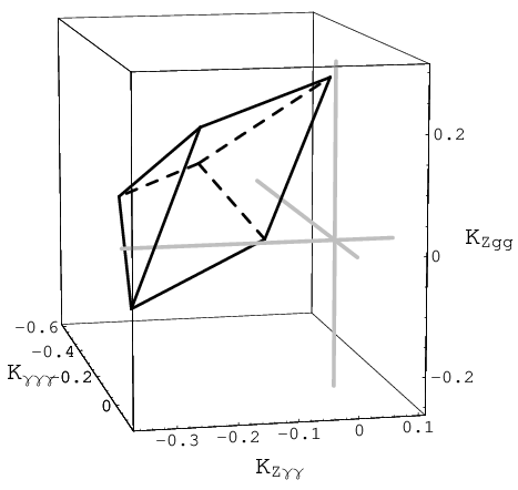
Fig.(1) shows the three-dimensional simplex that bounds allowed values for the dimensionless coupling constants ${\rm K}_{\gamma\gamma\gamma}$, ${\rm K}_{Z\gamma\gamma}$ and ${\rm K}_{Zgg}$. For any choosen point within the simplex in Fig.(1) the remaining coupling constants ${\rm K}_{ZZ\gamma}$, ${\rm K}_{ZZZ}$, ${\rm K}_{WW\gamma}$, ${\rm K}_{WWZ}$ and ${\rm K}_{\gamma gg}$ are uniquely fixed by the NCSM [6, 4]. This is true for any combination of three coupling constants.

Our total classical action reads

	$\displaystyle S_{cl}$	$\displaystyle=$	$\displaystyle S_{SM}+\sum_{i=1}^{3}S^{\theta}_{i}=g^{\prime 3}\kappa_{1}\theta^{\mu\nu}\int d^{4}x\left(\frac{a}{4}f_{\mu\nu}f_{\rho\sigma}f^{\rho\sigma}-f_{\mu\rho}f_{\nu\sigma}f^{\rho\sigma}\right)$		(22)
		$\displaystyle+$	$\displaystyle g^{\prime}g^{2}\kappa_{2}\theta^{\mu\nu}\int d^{4}x\left(\frac{a}{4}f_{\mu\nu}B_{\rho\sigma}^{i}B^{\rho\sigma i}-f_{\mu\rho}B_{\nu\sigma}^{i}B^{\rho\sigma i}+c.p.\right)$
		$\displaystyle+$	$\displaystyle g^{\prime}g^{2}_{S}\kappa_{3}\theta^{\mu\nu}\int d^{4}x\left(\frac{a}{4}f_{\mu\nu}G_{\rho\sigma}^{a}G^{\rho\sigma a}-f_{\mu\rho}G_{\nu\sigma}^{a}G^{\rho\sigma a}+c.p.\right).$

The term $S^{\theta}_{1}$ in (22) is one-loop renormalizable to linear order in $\theta$ [9] since the one-loop correction to the $S^{\theta}_{1}$ is of the second order in $\theta$. We need to investigate only the renormalizability of the remaining $S^{\theta}_{2}$ and $S^{\theta}_{3}$ parts of the action (22).

To realize the one-loop renormalization of the gauge part action (22), we apply, as before [9, 10], the background field method [15, 16]. As we have already explained the details of the method in [12], here we only discuss the points needed for this computation. The main contribution to the functional integral is given by the Gaussian integral. However, technically, this is achieved by splitting the vector potential into the classical-background plus the quantum-fluctuation parts, that is, $\phi_{V}\to\phi_{V}+{\bf\Phi}_{V}$, and by computing the terms quadratic in the quantum fields. In this way we determine the second functional derivative of the classical action, which is possible since our interactions (22) are of the polynomial type. The quantization is performed by the functional integration over the quantum vector field ${\bf\Phi}_{V}$ in the saddle-point approximation around the classical (background) configuration $\phi_{V}$.

First, an advantage of the background field method is the guarantee of covariance, because by doing the path integral the local symmetry of the quantum field ${\bf\Phi}_{V}$ is fixed, while the gauge symmetry of the background field ${\phi}_{V}$ is manifestly preserved.

Since we are dealing with gauge symmetry, our Lagrangian (22) is singular owing to its invariance under the gauge group. Therefore, a proper quantization of (22) requires the presence of the gauge fixing term $S_{\rm gf}[\phi]$, i.e. the Feynman-Fadeev-Popov ghost appears in the effective action

$$\Gamma[\phi]=S_{\rm cl}[\phi]+S_{\rm gf}[\phi]+\Gamma^{(1)}[\phi],\qquad S_{\rm gf}[\phi]=-\frac{1}{2}\int\mathrm{d}^{4}x(D_{\mu}{\bf\Phi}_{V}^{\mu})^{2}\;.$$

(23)

The one-loop effective part $\Gamma^{(1)}[\phi]$ is given by

$$\Gamma^{(1)}[\phi]=\frac{\mathrm{i}}{2}\log\det S^{(2)}[\phi]=\frac{\mathrm{i}}{2}{\rm Tr}\,\log S^{(2)}[\phi].$$

(24)

In (24), the $S^{(2)}[\phi]$ is the $2^{\rm nd}$-functional derivative of the classical action, with the following structure:

$$S^{2}=\Box+N_{1}+N_{2}+T_{2}+T_{3}+T_{4}\ .$$

(25)

Here $N_{1},N_{2}$ are commutative vertices, while $T_{2},T_{3},T_{4}$ are noncommutative ones. The indices denote the number of classical fields. The one-loop effective action computed by using the background field method is

	$\displaystyle\Gamma^{(1)}_{\theta,2}$	$\displaystyle=$	$\displaystyle\frac{\mathrm{i}}{2}{\rm Tr}\,\log\left({\cal I}+\Box^{-1}(N_{1}+N_{2}+T_{2}+T_{3}+T_{4})\right)$		(26)
			$\displaystyle\hskip-56.9055pt=\frac{\mathrm{i}}{2}\sum_{n=1}^{\infty}\frac{(-1)^{n+1}}{n}{\rm Tr}\,\left(\Box^{-1}N_{1}+\Box^{-1}N_{2}+\Box^{-1}T_{2}+\Box^{-1}T_{3}+\Box^{-1}T_{4}\right)^{n}\,.$

As the conventions and the notation are the same as in [10], we only encounter and discuss the final results.

The divergent one-loop vertex correction to (22) as a function of the SW freedom parameter $a$ is [10]

	$\displaystyle\Gamma_{\rm div}$	$\displaystyle=$	$\displaystyle\frac{11}{3(4\pi)^{2}\epsilon}\int d^{4}x\Big(B_{\mu\nu}^{i}B^{\mu\nu i}+\frac{3}{2}G_{\mu\nu}^{a}G^{\mu\nu a}\Big)$		(27)
		$\displaystyle+$	$\displaystyle\frac{4}{3(4\pi)^{2}\epsilon}{g^{\prime}}g^{2}\kappa_{2}(3-a)\theta^{\mu\nu}\int d^{4}x\big(\frac{1}{4}f_{\mu\nu}B_{\rho\sigma}^{i}-f_{\mu\rho}B_{\nu\sigma}^{i}\big)B^{\rho\sigma i}$
		$\displaystyle+$	$\displaystyle\frac{6}{3(4\pi)^{2}\epsilon}{g^{\prime}}g^{2}_{S}\kappa_{3}(3-a)\theta^{\mu\nu}\int d^{4}x\big(\frac{1}{4}f_{\mu\nu}G_{\rho\sigma}^{a}-f_{\mu\rho}G_{\nu\sigma}^{a}\big)G^{\rho\sigma a}\,.$

From (27) it is clear that the expanded gauge action (22) is renormalizable only for the value $a=3$ and, its noncommutative part is finite or free of divergencies, so the noncommutativity parameter $\theta$ need not be renormalized. The results for the bare fields and couplings, are given in [10].

Note that we have also analized the renormalizability properties of the pure NC SU(N) gauge sector, for vector fields in the adjoint representation [17]. We have found that this model is also renormalizable for $a=3$. However, to obtain renormalizability, we had to pay a price by necessity for the renormalization of the noncommutative deformation parameter $h$. In this way the parameter $h$ and/or the scale of noncommutativity $\Lambda_{\rm NC}$ become running quantities, dependent on energy [17].

In addition, it was shown that the one-loop contributions to the U(1) gauge-field part of the noncommutative gauge theories in the enveloping-algebra formalism are renormalizable at first order in $\theta$ even if the scalar matter, with and without spontaneous symmetry breaking, contributions are taken into account [18]. There is reasonable hope that the same conclusion should hold for SU(N), but the computations are expected to be extremely involving. Nevertheless, the results [18] further strengthen the philosophy which is embraced in our latest papers [10, 17].

From the action (22) we extract the triple-gauge boson terms which are not present in the commutative SM Lagrangian. In terms of the physical fields $A,\ W^{\pm},\ Z$, and $G$ they are

	$\displaystyle{\cal L}^{\theta}_{\gamma\gamma\gamma}$	$\displaystyle=$	$\displaystyle\frac{e}{4}\sin 2{\theta_{W}}\;{\rm K}_{\gamma\gamma\gamma}{\theta^{\rho\tau}}A^{\mu\nu}\left(aA_{\mu\nu}A_{\rho\tau}-4A_{\mu\rho}A_{\nu\tau}\right),$
	$\displaystyle{\rm K}_{\gamma\gamma\gamma}$	$\displaystyle=$	$\displaystyle\frac{1}{2}\;gg^{\prime}(\kappa_{1}+3\kappa_{2});$		(28)
	$\displaystyle{\cal L}^{\theta}_{Z\gamma\gamma}$	$\displaystyle=$	$\displaystyle\frac{e}{4}\sin 2{\theta_{W}}\,{\rm K}_{Z\gamma\gamma}\,{\theta^{\rho\tau}}$
		$\displaystyle\times$	$\displaystyle\left[2Z^{\mu\nu}\left(2A_{\mu\rho}A_{\nu\tau}-aA_{\mu\nu}A_{\rho\tau}\right)\right.+\left.8Z_{\mu\rho}A^{\mu\nu}A_{\nu\tau}-aZ_{\rho\tau}A_{\mu\nu}A^{\mu\nu}\right],$
	$\displaystyle{\rm K}_{Z\gamma\gamma}$	$\displaystyle=$	$\displaystyle\frac{1}{2}\;\left[{g^{\prime}}^{2}\kappa_{1}+\left({g^{\prime}}^{2}-2g^{2}\right)\kappa_{2}\right];$		(29)

where $A_{\mu\nu}\equiv\partial_{\mu}A_{\nu}-\partial_{\nu}A_{\mu}$, etc. The structure of the other interactions such as $ZZ\gamma$, $WWZ$, $ZZZ$, $Zgg$, and $\gamma gg$ is given in [4, 6].

Next we focus on the branching ratio of the $Z\rightarrow\gamma\gamma$ decay in the renormalizable model. Note that each term from the $\theta$-expanded action (22), (28) and (29) is manifestly invariant under the ordinary gauge transformations. The gauge-invariant amplitude ${\cal A}^{\theta}_{Z\rightarrow\gamma\gamma}$ for the $Z(k_{1})\rightarrow\gamma(k_{2})\,\gamma(k_{3})$ decay in the momentum space reads

$\displaystyle{\cal A}^{\theta}_{Z\to\gamma\gamma}=-2e\sin 2{\theta_{W}}{\rm K}_{Z\gamma\gamma}{\Theta^{\mu\nu\rho}_{3}}(a;k_{1},-k_{2},-k_{3})\epsilon_{\mu}(k_{1})\epsilon_{\nu}(k_{2})\epsilon_{\rho}(k_{3}).$

(30)

The tensor ${\Theta^{\mu\nu\rho}_{3}}(a;k_{1},k_{2},k_{3})$ is given by

	$\displaystyle{\Theta^{\mu\nu\rho}_{3}}(a;k_{1},k_{2},k_{3})$	$\displaystyle=$	$\displaystyle-\,(k_{1}\theta k_{2})\,$		(31)
		$\displaystyle\times$	$\displaystyle[(k_{1}-k_{2})^{\rho}g^{\mu\nu}+(k_{2}-k_{3})^{\mu}g^{\nu\rho}+(k_{3}-k_{1})^{\nu}g^{\rho\mu}]$
		$\displaystyle-$	$\displaystyle\theta^{\mu\nu}\,[k_{1}^{\rho}\,(k_{2}k_{3})-k_{2}^{\rho}\,(k_{1}k_{3})]$
		$\displaystyle-$	$\displaystyle\theta^{\nu\rho}\,[k_{2}^{\mu}\,(k_{3}k_{1})-k_{3}^{\mu}\,(k_{2}k_{1})]$
		$\displaystyle-$	$\displaystyle\theta^{\rho\mu}\,[k_{3}^{\nu}\,(k_{1}k_{2})-k_{1}^{\nu}\,(k_{3}k_{2})]$
		$\displaystyle+$	$\displaystyle(\theta k_{2})^{\mu}\,\left[g^{\nu\rho}\,k_{3}^{2}-k_{3}^{\nu}k_{3}^{\rho}\right]+(\theta k_{3})^{\mu}\,\left[g^{\nu\rho}\,k_{2}^{2}-k_{2}^{\nu}k_{2}^{\rho}\right]$
		$\displaystyle+$	$\displaystyle(\theta k_{3})^{\nu}\,\left[g^{\mu\rho}\,k_{1}^{2}-k_{1}^{\mu}k_{1}^{\rho}\right]+(\theta k_{1})^{\nu}\,\left[g^{\mu\rho}\,k_{3}^{2}-k_{3}^{\mu}k_{3}^{\rho}\right]$
		$\displaystyle+$	$\displaystyle(\theta k_{1})^{\rho}\,\left[g^{\mu\nu}\,k_{2}^{2}-k_{2}^{\mu}k_{2}^{\nu}\right]+(\theta k_{2})^{\rho}\,\left[g^{\mu\nu}\,k_{1}^{2}-k_{1}^{\mu}k_{1}^{\nu}\right]$
		$\displaystyle+$	$\displaystyle\theta^{\mu\alpha}(ak_{1}+k_{2}+k_{3})_{\alpha}\,\left[g^{\nu\rho}\,(k_{3}k_{2})-k_{3}^{\nu}k_{2}^{\rho}\right]$
		$\displaystyle+$	$\displaystyle\theta^{\nu\alpha}(k_{1}+ak_{2}+k_{3})_{\alpha}\,\left[g^{\mu\rho}\,(k_{3}k_{1})-k_{3}^{\mu}k_{1}^{\rho}\right]$
		$\displaystyle+$	$\displaystyle\theta^{\rho\alpha}(k_{1}+k_{2}+ak_{3})_{\alpha}\,\left[g^{\mu\nu}\,(k_{2}k_{1})-k_{2}^{\mu}k_{1}^{\nu}\right]\,,$

where the 4-momenta $k_{1},k_{2},k_{3}$ are taken to be incoming, satisfying the momentum conservation $(k_{1}+k_{2}+k_{3}=0)$. In (31) the freedom parameter $a$ appears symmetric in physical gauge bosons which enter the interaction point, as one would expect. The amplitude (30), for $a=3$, with the Z boson at rest gives the total rate for the $Z\rightarrow\gamma\gamma$ decay:

$\displaystyle\Gamma_{Z\rightarrow\gamma\gamma}$

$\displaystyle=$

$\displaystyle\frac{\alpha}{4}\;\frac{M^{5}_{Z}}{\Lambda^{4}_{\rm NC}}\;\sin^{2}2\theta_{W}{\rm K}^{2}_{Z\gamma\gamma}\big({\vec{E}}_{\theta}^{2}+{\vec{B}}_{\theta}^{2}\big),$

(32)

where ${\vec{E}}_{\theta}=\{{\theta}^{01},{\theta}^{02},{\theta}^{03}\}$ and ${\vec{B}}_{\theta}=\{{\theta}^{23},{\theta}^{31},{\theta}^{12}\}$ are dimensionless coefficients of order one, representing the time-space and space-space noncommutativity, respectively. For the $Z$ boson at rest, polarized in the direction of the third axis, we obtain the following polarized partial width:

$$\Gamma^{3}_{Z\rightarrow\gamma\gamma}=\frac{\alpha}{60}\frac{M^{5}_{Z}}{\Lambda^{4}_{\rm NC}}\sin^{2}2\theta_{W}{\rm K}^{2}_{Z\gamma\gamma}\left({\vec{E}}_{\theta}^{2}+{\vec{B}}_{\theta}^{2}+42\left((\theta^{03})^{2}+(\theta^{12})^{2}\right)\right)\,.$$

(33)

In order to estimate the scale of noncommutativity $\Lambda_{\rm NC}$ from $\Gamma_{Z\rightarrow\gamma\gamma}$,we consider new experimental possibilities at LHC. According to the CMS Physics Technical Design Report [19], around $10^{7}\;\,Z\to e^{+}e^{-}$ events are expected to be recorded with $10\;\,fb^{-1}$ of the data. From this one can estimate the expected number of $Z\to\gamma\gamma$ events per $10\;\,fb^{-1}$. Assuming that $BR(Z\to\gamma\gamma)\sim 10^{-8}$ and using $BR(Z\to e^{+}e^{-})=3\times 10^{-2}$, we may expect to have $\sim 3$ events of $Z\to\gamma\gamma$ with $10\;fb^{-1}$. Now the question is: What would be the background from $Z\to e^{+}e^{-}$ when the electron radiates a very high-energy bremsstrahlung photon in the beam pipe or in the first layer(s) of the Pixel Detector and is thus lost for the tracker reconstruction? In that case, the electron would not be reconstructed and would be misidentified as a photon. The probability of such an event should be evaluated from the full detector simulation. According to the CMS note [20] which studies the $Z\to e^{+}e^{-}$ background for $Higgs\to\gamma\gamma$, the probability to misidentify the electron as a photon is huge (see Fig. 3 in [20]) but the situation can be improved by applying more stringent selections to the photon candidate when searching for $Z\to\gamma\gamma$ events [21]. However, the irreducible di-photon background (Fig. 3 in [20]) might also kill the signal. In that case, one can only set the upper limits to the scale of noncommutativity from the $Z\to\gamma\gamma$ rate.

In accord with the analysis of the LHC experimental expectations [19, 20, 21] it is bona fide reasonable to assume that the lower bound for the branching ratio is $BR(Z\rightarrow\gamma\gamma)\stackrel{{\scriptstyle<}}{{\sim}}10^{-8}$. Next, choosing the lower central value of $|K_{Z\gamma\gamma}|=0.05$, from the figures and the Table in [6], we find that the upper bound to the scale of noncommutativity is $\Lambda_{\rm NC}\stackrel{{\scriptstyle>}}{{\sim}}1.0\;\,\rm TeV$ for ${\vec{E}}_{\theta}^{2}+{\vec{B}}_{\theta}^{2}\simeq 1$. The obtained bound is strongly supported in [18].

Clearly, the measurement of the $Z\rightarrow\gamma\gamma$ decay branching ratio would fix the quantity $|K_{Z\gamma\gamma}/\Lambda_{\rm NC}^{2}|$, while the inclusion of other triple gauge boson interactions through $2\to 2$ scattering experiments [14] would sufficiently reduce the available parameter space of our model by more precisely determining the relations among the couplings ${\rm K}_{\gamma\gamma\gamma}$, ${\rm K}_{Z\gamma\gamma}$, ${\rm K}_{ZZ\gamma}$, ${\rm K}_{ZZZ}$, ${\rm K}_{WW\gamma}$, and ${\rm K}_{WWZ}$. Next, we summarize our results and compare with those obtained previously.

The first $Z\to\gamma\gamma$ calculation [22] was performed within a different model which has different symmetries in comparison with ours and, because of the absence of the SW map, the model does not possess the commutative gauge invariance. Also, the $Z\to\gamma\gamma$ rate obtained in [22] by imposing the unitarity of the theory in the usual manner, $\theta^{0i}=0$, [23, 24], vanishes ³³ 3 The condition of unitarity can be covariantly generalized to $\theta_{\mu\nu}\theta^{\mu\nu}=2({\vec{B}}_{\theta}^{2}-{\vec{E}}_{\theta}^{2})>0$ [25]..

The partial width for the same process was obtained in [6] in the framework of similar theories, which, however, were not renormalizable. The present results for the partial widths $\Gamma_{Z\rightarrow\gamma\gamma}$ and $\Gamma^{3}_{Z\rightarrow\gamma\gamma}$ are about three times larger than those in [6] and consistently symmetric with respect to time-space and space-space noncommutativity. In the polarized rate (33) the third components ($(\theta^{03})^{2}+(\theta^{12})^{2}$) are enhanced relative to the other two components by a large factor, as expected. Also, the rate (33) is enhanced by a factor of $\sim$ 3 with respect to the total rate (32). The upper limit to the scale of noncommutativity $\Lambda_{\rm NC}\stackrel{{\scriptstyle>}}{{\sim}}1$ TeV is significantly higher than in [6]. This bound is now firmer owing to the regular behavior of the triple gauge boson interactions (28-29) with respect to the one-loop renormalizability of the NCSM gauge sector.

After 10 years of the LHC running the integrated luminosity is expected to reach $\sim 1000\;\,fb^{-1}$, [20]. This means that for the assumed $BR(Z\to\gamma\gamma)\sim 10^{-8}$ we should have $\sim 300$ events of $Z\to\gamma\gamma$, that is we should be well above the background. On the other hand, this result can also be understood as $\sim 3$ events with the $BR(Z\to\gamma\gamma)\sim 10^{-10}$, which lifts the scale of noncommutativity up by a factor of $\sim 3$. Therefore, with a more stringent selection of photon candidates and if the irreducible di-photon contamination becomes controllable, the $Z\rightarrow\gamma\gamma$ decay will become a clean signature of space-time noncommutativity in LHC experiments.

Finally, the results of [17,18], while strongly supporting this computations, might also hint at the existence of new interaction symmetry of the noncommutative gauge sector. Such new symmetry could be a responsible for the renormalizability of the noncommutative matter sector including fermions and, next, for the main goal, i.e. in general, the physical realization of the Lorentz invariance breaking at very high energies, respectively.

References

- [1] N. Seiberg and E. Witten, String theory and non-commutative geometry, JHEP 09 (1999) 032 [arXiv:hep-th/9908142].
- [2] J. Madore, S. Schraml, P. Schupp and J. Wess, Gauge theory on non-commutative spaces, Eur. Phys. J. C16 (2000) 161 [arXiv:hep-th/0001203]; B. Jurčo, S. Schraml, P. Schupp and J. Wess, Enveloping algebra valued gauge transformations for non-Abelian gauge groups on non-commutative spaces, Eur. Phys. J. C17 (2000) 521 [arXiv:hep-th/0006246]; B. Jurčo, L. Möller, S. Schraml, P. Schupp and J. Wess, Construction of non-Abelian gauge theories on non-commutative spaces, Eur. Phys. J. C21 (2001) 383 [arXiv:hep-th/0104153].
- [3] X. Calmet, B. Jurčo, P. Schupp, J. Wess and M. Wohlgenannt, The standard model on non-commutative space-time, Eur. Phys. J. C23 (2002) 363 [arXiv:hep-ph/0111115].
- [4] B. Melic, K. Passek-Kumericki, J. Trampetic, P. Schupp and M. Wohlgenannt, The standard model on non-commutative space-time: Electroweak currents and Higgs sector, Eur. Phys. J. C 42 (2005) 483 [arXiv:hep-ph/0502249]. B. Melic, K. Passek-Kumericki, J. Trampetic, P. Schupp and M. Wohlgenannt, The standard model on non-commutative space-time: Strong interactions included, Eur. Phys. J. C 42 (2005) 499 [arXiv:hep-ph/0503064].
- [5] P. Aschieri, B. Jurčo, P. Schupp and J. Wess, Non-Commutative GUTs, Standard Model and C,P,T, Nucl. Phys. B651 (2003) 45 [arXiv:hep-th/0205214].
- [6] W. Behr, N.G. Deshpande, G. Duplančić, P. Schupp, J. Trampetić and J. Wess, The Z Decays in the Noncommutative Standard Model, Eur. Phys. J. C29 (2003) 441 [arXiv:hep-ph/0202121]; G. Duplančić, P. Schupp and J. Trampetić, Comment on triple gauge boson interactions in the non-commutative electroweak sector, Eur. Phys. J. C32 (2003) 141 [arXiv:hep-ph/0309138].
- [7] M. Buric, D. Latas, V. Radovanovic and J. Trampetic, Improved Z decay in the renormalizable gauge sector of the non-commutative standard model, [arXiv:hep-ph/0611299].
- [8] F. Brandt, C.P. Martin and F. Ruiz Ruiz, Anomaly freedom in Seiberg-Witten non-commutative gauge theories, JHEP 07 (2003) 068 [arXiv:hep-th/0307292].
- [9] M. Buric, D. Latas and V. Radovanovic, Renormalizability of non-commutative SU(N) gauge theory, JHEP 0602 (2006) 046 [arXiv:hep-th/0510133].
- [10] M. Buric, V. Radovanovic and J. Trampetic, The one-loop renormalization of the gauge sector in the -expanded non-commutative standard model, JHEP 03 (2007) 030 [arXiv:hep-th/0609073].
- [11] R. Wulkenhaar, Non-Renormalizability Of Theta-Expanded Noncommutative QED, JHEP 0203 (2002) 024 [arXiv:hep-th/0112248].
- [12] M. Buric and V. Radovanovic, Non-renormalizability of non-commutative SU(2) gauge theory, JHEP 0402 (2004) 040 [arXiv:hep-th/0401103];
- [13] J. Trampetić, Rare and forbidden decays, Acta Phys. Polon. B33 (2002) 4317 [hep-ph/0212309]; B. Melic, K. Passek-Kumericki and J. Trampetic, Quarkonia decays into two photons induced by the space-time non-commutativity, Phys. Rev. D 72 (2005) 054004 [arXiv:hep-ph/0503133]; K pi gamma decay and space-time non-commutativity, Phys. Rev. D 72 (2005) 057502 [arXiv:hep-ph/0507231];
- [14] A. Alboteanu, T. Ohl and R. Ruckl, Collider tests of the non-commutative standard model, PoS HEP2005 (2006) 322 [arXiv:hep-ph/0511188]; Probing the non-commutative standard model at hadron collider, Phys. Rev. D 74, 096004 (2006) [arXiv:hep-ph/0608155].
- [15] G. ’t Hooft, An algorithm for the poles at dimension four in the dimensional regularization procedure, Nucl. Phys. B 62 (1973) 444.
- [16] M. E. Peskin and D. V. Schroeder, An introduction to Field Theory, Perseus Books, Reading 1995.
- [17] D. Latas, V. Radovanovic and J. Trampetic, Non-commutative SU(N) gauge theories and asymptotic freedom, arXiv:hep-th/0703018.
- [18] C. P. Martin, D. Sanchez-Ruiz and C. Tamarit, The noncommutative U(1) Higgs-Kibble model in the enveloping-algebra formalism and its renormalizability, arXiv:hep-th/0612188.
- [19] CMS Physics Technical Design Report, Vol.1. CERN/LHCC 2006-001.
- [20] M. Pieri et al., CMS Note 2006/112.
- [21] A. Nikitenko, private communications.
- [22] I. Mocioiu, M. Pospelov and R. Roiban, Low-energy limits on the antisymmetric tensor field background on the brane and on the non-commutative scale, Phys. Lett. B 489, 390 (2000) [arXiv:hep-ph/0005191];
- [23] N. Seiberg, L. Susskind and N. Toumbas, Space/time non-commutativity and causality, JHEP 0006, 044 (2000) [arXiv:hep-th/0005015].
- [24] J. Gomis and T. Mehen, Space-time noncommutative field theories and unitarity, Nucl. Phys. B 591, 265 (2000) [arXiv:hep-th/0005129].
- [25] S. M. Carroll, J. A. Harvey, V. A. Kostelecky, C. D. Lane and T. Okamoto, Noncommutative field theory and Lorentz violation, Phys. Rev. Lett. 87, 141601 (2001) [arXiv:hep-th/0105082].