$q$-deformed spin foam models of quantum gravity

The Lie algebra $\mathfrak{su}(2)$ is generated by the well known Pauli matrices $\sigma_{i}$, which obey the commutation relations

where $\sigma_{\pm}=\sigma_{1}\pm i\sigma_{2}$. The universal enveloping algebra of $\mathfrak{su}(2)$ is the associative algebra generated by $\sigma_{\pm}$ and $\sigma_{3}$ subject to the above identities, with the Lie bracket being interpreted as $[A,B]=AB-BA$.

The $q$-deformed algebra $\mathfrak{su}_{q}(2)$ is constructed by replacing $\sigma_{3}$ with another generator. Formally, it is thought of as $\Sigma=q^{\frac{1}{2}\sigma_{3}}$, where $q\in\mathbb{C}$ with the exceptions $q\neq 0,1,-1$. The Lie bracket relations are replaced by the identities

We can rewrite $q=1+2\varepsilon$ and think of $\varepsilon$ as a small complex number. Then, formally at leading order in $\varepsilon$, the substitution $\Sigma=q^{\frac{1}{2}\sigma_{3}}=1+\varepsilon\sigma_{3}+O(\varepsilon^{2})$ reduces the deformed identities (2) to the standard Lie algebra relations (1). The associative algebra generated by $\sigma_{\pm}$ and $\sigma_{3}$ subject to the deformed identities (2) is the algebra $\mathfrak{su}_{q}(2)$.

For generic $q$, that is, when $q$ is not a root of unity, the finite-dimensional irreducible representations of $\mathfrak{su}_{q}(2)$ are classified by a half-integer, $j=0,1/2,1,3/2,\ldots,$ referred to as the spin, in direct analogy with the representations of $\mathfrak{su}(2)$ and the theory of angular momentum. The dimension of the representation $j$ is $2j+1$. When $q=\exp(i\pi/r)$ is a $2r$th root of unity (ROU), where $r>2$ is an integer called the ROU parameter, the representations $j$ are still defined, but become reducible for $j>(r-2)/2$. They decompose into a sum of representations with spin at most $(r-2)/2$ and so-called trace 0 ones, whose nature will be explained below.

For the purposes of this paper we are concerned only with intertwiners between representations of $\mathfrak{su}_{q}(2)$, i.e., linear maps commuting with the action of the algebra, and their (quantum) traces¹¹ 1 When $q=1$, this notion of trace reduces up to sign to the usual trace of a linear map, but is slightly different otherwise, cf. [CFS]*Chapter 4..

Any such intertwiner can be constructed from a small set of generators and elementary operations on them. These constructions, as well as traces, can be represented graphically. Such graphs are called (abstract) spin networks. Their calculus is well developed and is described in [KL], whose conventions we follow throughout the paper with one exception: we use spins (half-integers) instead of twice-spins (integers). A brief review of our notation and conventions can be found in the Appendix.

Trace 0 representations of $\mathfrak{su}_{q}(2)$ are so called because the trace of an intertwiner from such a representation to itself is always zero. Thus, they can be freely discarded, as they do not contribute to the evaluation of $q$-deformed spin networks.

Deformation, especially with $q=\exp(i\pi/r)$ a $2r$th primitive ROU, is important for spin foam models for at least two reasons. Replacing $q=1$ by some ROU can act as a regulator for a model whose partition function and observable values are otherwise divergent. Also, $\mathfrak{su}_{q}(2)$ spin networks²² 2 These are graphs embedded in a $3$-manifold, labelled by representations of $\mathfrak{su}_{q}(2)$. They are similar to but distinct from the abstract spin networks referred to above. See [Baez] for the distinction. naturally appear when considering a positive cosmological constant in loop quantum gravity.

The original Ponzano-Regge model [PR] attempts to express the path integral for $3$-dimensional Riemannian general relativity as a sum over labelled triangulations of a $3$-manifold. The edges of the triangulation are labelled by discrete lengths, identified with spin labels of irreducible $SU(2)$ representations. Each tetrahedron contributes a $6j$-symbol factor to the summand, normalized to ensure invariance of the overall sum under change of triangulation. Unfortunately, the Ponzano-Regge model turned out to be divergent. Motivated by the construction of $3$-manifold invariants, Turaev and Viro were able to regularize the Ponzano-Regge model [TV, AW] by replacing the $SU(2)$ $6j$-symbols with their $q$-deformed analogs at a ROU $q$. The key feature of the regularization is the truncation of the summation to only the irreducible representations of $\mathfrak{su}_{q}(2)$ of non-zero trace, which leaves only a finite number of terms in the model’s partition function.

A version of the Barrett-Crane model, derived from a group field theory by De Pietri, Freidel, Krasnov and Rovelli [DFKR] (DFKR for short), was also found to be divergent. A $q$-deformed version of the same model at a ROU $q$ is similarly regularized (see Section 3.2). Some numerical results for the regularized version of this model are given in Section 5.2.

The argument linking $q$-deformation to the presence of a positive cosmological constant is due to Smolin [Smolin] and is given in more refined form in [Smolin-posCC]. It is briefly summarized as follows. Loop quantum gravity begins by writing the degrees of freedom of general relativity in terms of an $SU(2)$ connection on a spatial slice and the slice’s extrinsic curvature. A state in the Schrödinger picture, a wave function on the space of connections, can be constructed by integrating the Chern-Simons $3$-form over the spatial slice. This state, known as the Kodama state, simultaneously satisfies all the canonical constraints of the theory and semiclassically approximates de Sitter spacetime, which is a solution of the vacuum Einstein equations with a positive cosmological constant. The requirement that the Kodama state also be invariant under large gauge transformations implies discretization of the cosmological constant, $\Lambda\sim 1/r$, with $r$ a positive integer. The coefficients of the Kodama state in the spin network basis are obtained by evaluating the labelled graph, associated to a basis state, as an abstract $\mathfrak{su}_{q}(2)$ spin network. Here the deformation parameter $q$ is a ROU, $q=\exp(i\pi/r)$, where the ROU parameter $r$ is identified with the discretization parameter of the cosmological constant.

Given the heuristic link [Baez] between spin networks of loop quantum gravity and spin foams, it is natural to $q$-deform a spin foam model as an attempt to account for a positive cosmological constant. With this aim, Noui and Roche [NR] have given a $q$-deformed version of the Lorentzian Barrett-Crane model. The possibility of $q$-deformation has been with the Riemannian Barrett-Crane model since its inception [BC-riem] and all the necessary ingredients have been present in the literature for some time. In the next section these details are collected in a form ready for numerical investigation.

The Riemannian Barrett-Crane model was first proposed in [BC-riem]. Its relation to the Crane-Yetter [CY] spin foam model is analogous to the relation of the Plebanski [Plebanski] formulation of general relativity (GR) to $4$-dimensional $BF$ theory with $\mathrm{Spin}(4)$ as the structure group. Both $BF$ theory and the Crane-Yetter model are topological and the latter is considered a quantization of the former [CY-BF]. In the Plebanski formulation, GR is a constrained version of $BF$ theory. Similarly, the Barrett-Crane model restricts the spin labels summed over in the Crane-Yetter model. With this restriction, Barrett and Crane hoped to produce a discrete model of quantum (Riemannian) GR.

Thanks to graphical notation, the $q$-deformation of the spin foam amplitudes described above is straightforward, with only a few subtleties. The main distinction is that $q$-deformed graphs are actually ribbon (framed) graphs with braiding. Thus, any undeformed spin network has to be supplemented with information about twists and crossings before evaluation.

In [Yetter], Yetter generalized the Barrett-Crane $4$-vertex for a $q$-deformed version of $\mathfrak{spin}(4)$. Since $\mathfrak{spin}(4)\cong\mathfrak{su}(2)\oplus\mathfrak{su}(2)$, there is a two parameter family of possible deformations of the Lie algebra, $\mathfrak{spin}_{q,q^{\prime}}(4)\cong\mathfrak{su}_{q}(2)\oplus\mathfrak{su}_{q^{\prime}}(2)$. Yetter singles out the one parameter family $q^{\prime}=q^{-1}$, restricted to balanced representations, since it preserves the invariance of the Barrett-Crane vertex under rotations. This family also has especially simple curl and twist identities:

$$\raisebox{-17.0141pt}{\hbox{\begin{picture}\includegraphics[]{curl.pstex}\end{picture}\begin{picture}(1.0,-122.0)\put(91.0,839.0){\pic@makebox@{\makebox}{}(0.0,0.0)[lb]{\smash{{{\color[rgb]{0,0,0}$j$}}}}}\end{picture}}}\phantom{j}=\phantom{jj}\raisebox{-17.0141pt}{\hbox{\begin{picture}\includegraphics[]{line.pstex}\end{picture}\begin{picture}(1.0,-114.0)\put(136.0,839.0){\pic@makebox@{\makebox}{}(0.0,0.0)[lb]{\smash{{{\color[rgb]{0,0,0}$j$}}}}}\end{picture}}}\phantom{j\otimes}\quad\text{and}\quad\phantom{a\otimes}\raisebox{-17.0141pt}{\hbox{\begin{picture}\includegraphics[]{3-vert-braid-dot.pstex}\end{picture}\begin{picture}(-37.0,-211.0)\put(249.0,-196.0){\pic@makebox@{\makebox}{}(0.0,0.0)[b]{\smash{{{\color[rgb]{0,0,0}$c$}}}}}\put(-22.0,749.0){\pic@makebox@{\makebox}{}(0.0,0.0)[rb]{\smash{{{\color[rgb]{0,0,0}$a$}}}}}\put(518.0,749.0){\pic@makebox@{\makebox}{}(0.0,0.0)[lb]{\smash{{{\color[rgb]{0,0,0}$b$}}}}}\end{picture}}}\phantom{b\otimes b}=\phantom{a\otimes a}\raisebox{-17.0141pt}{\hbox{\begin{picture}\includegraphics[]{3-vert-dot.pstex}\end{picture}\begin{picture}(-14.0,-211.0)\put(361.0,-196.0){\pic@makebox@{\makebox}{}(0.0,0.0)[b]{\smash{{{\color[rgb]{0,0,0}$c$}}}}}\put(721.0,749.0){\pic@makebox@{\makebox}{}(0.0,0.0)[lb]{\smash{{{\color[rgb]{0,0,0}$b$}}}}}\put(1.0,749.0){\pic@makebox@{\makebox}{}(0.0,0.0)[rb]{\smash{{{\color[rgb]{0,0,0}$a$}}}}}\end{picture}}}\phantom{b\otimes},$$

(11)

where the left factor of $j\otimes j$ corresponds to $\mathfrak{su}_{q}(2)$ and the right one to $\mathfrak{su}_{q^{-1}}(2)$, and the $3$-vertex is the obvious juxtaposition of two $\mathfrak{su}_{q}(2)$ and $\mathfrak{su}_{q^{-1}}(2)$ $3$-vertices. Once this deformation is adopted, the ribbon structure can be ignored [Yetter], so one only needs to specify the crossing structure for a given $\mathfrak{spin}(4)$ spin network to obtain a well-defined $q$-evaluation.

There are three basic graphs needed to define the Barrett-Crane simplex amplitudes: the bubble, the eye, and the $10j$-symbol. The evaluation of the bubble graph, Equation (9), is $[2j+1]^{2}$, where the quantum integer $[2j+1]$ is defined in the Appendix. Remarkably, the value of the eye diagram turns out not to depend on $q$ and its value is still given by Equation (10). The only exception is when $q$ is a ROU with parameter $r$. Then, the dimension of the space of $4$-valent intertwiners changes to

$$\raisebox{-17.0141pt}{\hbox{\begin{picture}\includegraphics[]{eye.pstex}\end{picture}\begin{picture}(1.0,-122.0)\put(496.0,119.0){\pic@makebox@{\makebox}{}(0.0,0.0)[b]{\smash{{{\color[rgb]{0,0,0}$j_{4}$}}}}}\put(496.0,322.0){\pic@makebox@{\makebox}{}(0.0,0.0)[b]{\smash{{{\color[rgb]{0,0,0}$j_{3}$}}}}}\put(496.0,546.0){\pic@makebox@{\makebox}{}(0.0,0.0)[b]{\smash{{{\color[rgb]{0,0,0}$j_{2}$}}}}}\put(496.0,772.0){\pic@makebox@{\makebox}{}(0.0,0.0)[b]{\smash{{{\color[rgb]{0,0,0}$j_{1}$}}}}}\end{picture}}}=\begin{cases}\min\left\{\begin{matrix}\phantom{r-{}}1+\min\{2j,s-2J\}\\ r-1-\max\{2J,s-2j\}\end{matrix}\right\}&\parbox{65.00009pt}{if positive and\\ $s$ is integral,}\\ 0&\text{otherwise,}\end{cases}$$

(12)

where again $s=\sum_{k}j_{k}$, $j=\min_{k}j_{k}$, and $J=\max_{k}j_{k}$.

The $10j$-symbol is the only network with a non-planar graph. Originally, it was defined in terms of the $15j$-symbol from the Crane-Yetter model. This $15j$-symbol was defined with $q$-deformation in mind, so its crossing and ribbon structure was fully specified [CKY]*Section 3. Adapted to the $10j$-graph, it can be summarized as follows: Consider a $4$-simplex. The dual 1-skeleton of the boundary has five dual vertices and ten dual edges, and is the complete graph $K_{5}$ on these five dual vertices. If we remove one of the (non-dual) vertices from the boundary of the $4$-simplex, what remains is homeomorphic to $\mathbb{R}^{3}$. For any such homeomorphism, the embedding of $K_{5}$ into $\mathbb{R}^{3}$ can be projected onto a $2$-dimensional plane. The crossing structure of the $10j$ graph is defined by such a projection. It is illustrated in Equation (5). Although, with crossings, the $10j$ graph is no longer manifestly invariant under permutations of its vertices, it can be shown to be so.

The definition of observables in a spin foam model of quantum gravity is still open to interpretation (see Section 6 of [BCHT] for a brief discussion). For a fixed spin foam, the half-integer spin labels of its faces are the fundamental variables of the model. Practically speaking, any observable of a spin foam model should be an expectation value of some function $O(F)$ of the spin labels of a spin foam $F$, averaged over all spin foams with amplitudes specified by Equation (3):

In this paper we choose to concentrate on a few observables representative of the kind of quantities computable in a spin foam model. As before, fix a triangulation of a $4$-manifold, let $\Delta_{2}$ represent the set of its faces and let $j\colon\Delta_{2}\to\{0,1/2,1,\ldots\}$ be the spin labelling. We define:

where $\left\lfloor{n}\right\rceil$ denotes a quantum half-integer (see Appendix), $|\cdot|$ denotes cardinality, $\mathrm{dist}(f,f^{\prime})$ denotes the distance between faces, and $N_{d}$ is a normalization factor (see below for the definition of distance and $N_{d}$). These observables represent average spin per face, variance of spin per face, average area per face, and spin-spin correlation as a function of $d$.

The choice of observables given above is somewhat arbitrary. For instance, there are several subtly distinct choices for the expression for $(\delta J)^{2}$. Fortunately, they all yield expectation values that are nearly identical. The expression given above has the technical advantage of falling into the class of so-called single spin observables. These are observables whose expectation value can be directly obtained from the knowledge of probability with which spin $j$ occurs on any face of a spin foam. All of $J$, $(\delta J)^{2}$, and $A$ are single spin observables, while $C_{d}$ is not.

Note that on a fixed triangulation with no other background geometry, there is no physical notion of distance. We can, instead, define a combinatorial analog. For any two faces $f$ and $f^{\prime}$ of a given triangulation, let $\mathrm{dist}(f,f^{\prime})$ be the smallest number of face-sharing tetrahedra that connect $f$ to $f^{\prime}$. Given the discrete structure of our spacetime model, it is conceivable that this combinatorial distance, multiplied by a fundamental unit of length, approximates some notion of distance derived from the dynamical geometry of the spin foam model.

The correlation function $C_{d}$ may be thought of as analogous to a normalized $2$-point function of quantum field theory. The $d$-degree of face $f$ is the number of faces $f^{\prime}$ such that $\mathrm{dist}(f,f^{\prime})=d$. If the $d$-degree of every face is the same, the normalization factor $N_{d}$ can be taken to be the number of terms in the sum (17), that is, the number of face pairs separated by distance $d$. This choice ensures the inequality $|C_{d}|\leq 1$. If not all faces have the same $d$-degree, then the normalization factor has to be modified to

where $D_{d}$ is the maximum $d$-degree of a face, which reduces to the simpler definition in the case of uniform $d$-degree.

The choice of the $q$-dependent expression $\left\lfloor{j}\right\rceil$, instead of simply using the half-integer $j$, is motivated in Section 5.1. For some $q$, the argument of the square root in $A(F)$ may be negative or even complex. In that case, a branch choice will have to be made. Luckily, if $q=1$, $q$ is a ROU, or $q$ is real, the expression under the square root is always non-negative.

The derivation of the Christensen-Egan algorithm given in [CE] is contingent on the possibility of splitting the Barrett-Crane $4$-vertex as in Equation (4) and on the recoupling identity, Equation (43) of the Appendix. Both identities still hold in the $q$-deformed case. The validity of the $4$-vertex splitting was proved by Yetter [Yetter] and the recoupling identity is a standard part of $\mathfrak{su}_{q}(2)$ representation theory.

The only remaining detail of the algorithm’s generalization is the crossing structure of the $10j$ graph, which was established in Section 3.2. However, its only consequence is an extra factor from the twist implicit in the bubble diagram of Section 4 of [CE], cf. Equation (50) of the Appendix. We will not reproduce the derivation of the algorithm here. However, the way in which the twist arises is schematically illustrated in Figure 1. Note that the triviality of the twist for Yetter’s balanced representations, Equation (11), does not apply here since the twist occurs separately in distinct $\mathfrak{su}_{q}(2)$ networks.

The algorithm itself can be summarized in the following form:

The $10j$-symbol depends on the ten spins $j_{i,k}$, ($i=1,2$, $k=0,\ldots,4$) specified in Equation (5). The overall prefactor depends on the total spin $S=\sum_{i,k}j_{i,k}$ and the per-term prefactor is

The exponents of $(-)$ and $q$ are always integers. The $M_{k}$ are matrices (not all of the same size) of dimensions compatible with the five-fold product and trace. Their matrix elements are

The quantum integers $[n]$, as well as the theta $\theta(a,b,c)$ and tetrahedral $\operatorname{Tet}[{\cdots}]$ $\mathfrak{su}_{q}(2)$ spin networks are defined in the Appendix.

The quantities $l_{k}$ and $m_{i}$ are spin labels (half-integers). They are constrained by admissibility conditions (parity conditions and triangle inequalities). The parity of each index is determined by the conditions

for $i=1,2$ and $k=0,\ldots,4$, where $\equiv$ denotes equivalence mod $1$ and the second subscript of $j$ is taken mod $5$. Summation bounds are determined by the triangle inequalities, which must be checked for each trivalent vertex introduced in the derivation of the algorithm. They boil down to

for $i=1,2$ and $k=0,\ldots,4$, where we have used the notation

When $q=\exp(i\pi/r)$ is a ROU, extra inequalities must be taken into account to exclude summation over reducible representations. These are

where now

If any of the parity constraints or inequalities cannot be satisfied, the $10j$-symbol evaluates to zero.

This algorithm has been implemented and tested in the $q=1$ and ROU cases, for both $j$ and $r$ up to several hundreds. Unfortunately, for generic $q$, when $Q=\max\{|q|,|q|^{-1}\}>1$, the quantum integers grow exponentially as $|[n]|\sim Q^{n}$. Such a rapid growth makes the sums involved in this algorithm numerically unstable. It is still possible to use this algorithm with $Q$ close to $1$ or symbolically, using rational functions of $q$ instead of limited precision floating point numbers. Symbolic computation is, however, significantly slower (by up to a factor of $10^{6}$) than its floating point counterpart. The software library spinnet which implements these and other spin network evaluations is available from the authors and will be described in a future publication.

The sums involved in evaluating expectation values of observables, as in Equation (13), are very high-dimensional. For instance, a minimal triangulation of the $4$-sphere (seen as the boundary of a $5$-simplex) contains $20$ faces. Hence, any brute force evaluation of an expectation value, even on such a small lattice, involves a sum over the $20$-dimensional space of half-integer spin labels.

Fortunately, in the undeformed case, the total amplitude $Z(F)$ for a closed spin foam is never negative³³ 3 We expect the same thing to hold in Lorentzian signature [BC-pos, CC]. [BC-pos]. The proof for the $q=1$ case generalizes to the ROU case. One need only realize two facts. The first is that, in the ROU case, quantum integers are non-negative. The second is that, for $q$ a ROU, an $\mathfrak{su}_{q^{-1}}(2)$ spin network evaluates to the complex conjugate of the corresponding $\mathfrak{su}_{q}(2)$ spin network. The disjoint union of any two such spin networks evaluates to their product, the absolute value squared of either of them, and hence is non-negative. Then, the same positivity result follows as from Equation (1) of [BC-pos]. This positivity allows us to treat $Z(F)$ as a statistical distribution and use Monte Carlo methods to extract expectation values with much greater efficiency than brute force summation.

The main tool for evaluating expectation values is the Metropolis algorithm [Metrop, LB]. The algorithm consists of a walk on the space of spin labellings. Each step is randomly picked from a set of elementary moves and is either accepted or rejected based on the relative amplitudes of spin foam configurations before and after the move. An expectation value is extracted as the average of the observable over the configurations constituting the walk. Elementary moves for spin foam simulations are discussed in the next section.

A Metropolis-like algorithm is possible even if individual spin foam amplitudes $Z(F)$ are negative or even complex. However, if the total partition function $Z_{\mathrm{tot}}$ sums to zero, then the expectation values in Equation (13) become ill defined. Moreover, in numerical simulations, if $Z_{\mathrm{tot}}$ is even close to zero, expectation value estimates may exhibit great loss of precision and slow convergence. In the path-integral Monte Carlo literature, this situation is known as the sign problem [sgn-prob]. Still, the sign problem need not occur or, depending on the severity of the problem, there may be ways of effectively dealing with it.

Independent Metropolis runs can be thought of as providing independent estimates of a given expectation value. Thus, the error in the computed value of an observable can be estimated through the standard deviation of the results of many independent simulation runs [KI].

The choice of elementary moves for spin foam simulations must satisfy several criteria. Theoretically, the most important one is ergodicity. That is, any spin foam must be able to transform into any other one through a sequence of elementary moves which avoid configurations with zero amplitude. Practically, it is important that these moves usually preserve admissibility. A spin foam $F$ is called admissible if the associated amplitude $Z(F)$ is non-zero. If, starting with an admissible spin foam, most elementary moves produce an inadmissible spin foam, the simulation will spend a lot of time rejecting such moves without any practical benefit.

As before, consider a fixed triangulation of a compact $4$-manifold. The parity conditions (23) imposed on the $j_{i,k}$,

when taken together with the total spin foam amplitude (3), provide strong constraints on admissible spin foams. One can show that a move that changes spin labels by $\pm 1/2\pmod{1}$ on each face of a closed surface in the dual $2$-skeleton preserves the parity constraint. We take as the elementary moves the moves that change the spin labels by $\pm 1/2$ on the boundaries of the dual $3$-cells of the dual $3$-complex; the dual $3$-cells correspond to the edges of the triangulation. If the manifold has non-trivial mod $2$ homology in dimension $2$, additional moves would be necessary, but for the examples we consider the moves above suffice. From a practical point of view, extra moves might improve the simulation’s equilibration time. For instance, in the ROU case, parity preserving moves that change the spins from $0$ to $(r-2)/2$ or $(r-3)/2$ were introduced, since spins close to either admissible extreme may have large amplitudes. This property of the Perez-Rovelli and Baez-Christensen models is illustrated in the following section.

Unfortunately, the inequalities constraining spin labels do not have a similar geometric interpretation and cannot be used to easily restrict the set of elementary moves in advance.

The most striking result we can report is a discontinuity in the transition to the limit $r\to\infty$, where $r$, a positive integer, is the ROU parameter with $q=\exp(i\pi/r)$. As $r\to\infty$, the deformation parameter $q$ tends to its classical value $1$. If we interpret the cosmological constant as inversely proportional to $r$, $\Lambda\sim 1/r$, this limit also corresponds to $\Lambda\to 0$, through positive values. For a fixed spin foam, the amplitudes and observables we study tend continuously to their undeformed values as $r\to\infty$. However, we find that observable expectation values do not tend to their undeformed values in the same limit, that is, $\left\langle{O}\right\rangle_{r}\nrightarrow\left\langle{O}\right\rangle_{q=1}$ as $r\to\infty$.

The discontinuity is most simply illustrated with the single spin distribution, that is the probability of finding spin $j$ at any spin foam face. This probability can be estimated from the histogram of all spin labels that have occurred during a Monte Carlo simulation. The points in Figure 2(a)

show the single spin distributions for the Baez-Christensen model with $r=50$ and $q=1$. The curves show the corresponding single bubble amplitude. It is the amplitude $Z(F_{j})$ of a spin foam $F_{j}$ with all spin labels zero, except for the boundary of an elementary dual $3$-cell, whose faces are all labelled with spin $j$. The amplitudes and distributions are normalized as probability distributions so their sums over $j$ yield $1$. The similarity between the points and the continuous curves is consistent with the hypothesis that spin foams with isolated bubbles dominate the partition function sum. The behavior of the single spin distribution for the Perez-Rovelli model is very similar, except that its peaks are much more pronounced.

Note that the undeformed single spin distribution has a single peak at $j=0$, while the $r=50$ case has two peaks, one at $j=0$ and the other at $j=(r-2)/2$, the largest non-trace 0 irreducible representation. The bimodal nature of the single spin distribution has an important impact on the large $r$ behavior of observable expectation values, as is most easily seen with single spin observables (Section 3.3). For instance, if we consider the average, $\bar{j}$, of the half-integers $j$, the large $j$ peak would dominate the expectation value and $\left\langle{\bar{j}}\right\rangle$ would diverge linearly in $r$, as $r\to\infty$. On the other hand, since $J$ is the average of the quantum half-integers $\left\lfloor{j}\right\rceil$, $\left\langle{J}\right\rangle$ at least approaches a constant in the same limit. This is illustrated in Figure 2(b).

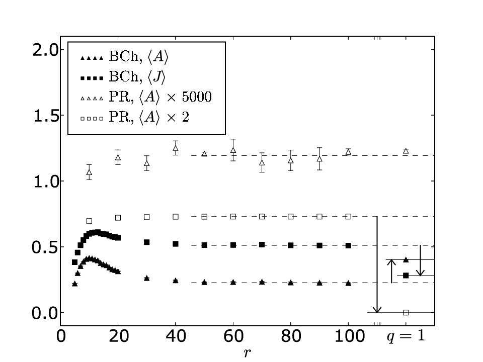
However, as shown in Figure 3, this limit is not the same as the undeformed expectation value. At the same time, as can be seen from the plot of the Perez-Rovelli average area in the same figure, there are some observables whose large $r$ limits are at least very close to the undeformed values. The area observable summand $A_{j}=\sqrt{\left\lfloor{j}\right\rceil\left\lfloor{j+1}\right\rceil}$ is exactly zero at both $j=0$ and $j=(r-2)/2$, while the spin observable summand $J_{j}=\left\lfloor{j}\right\rceil$ is zero at $j=0$ but still positive at $j=(r-2)/2$, Figure 2(b). The large $j$ peak of the Perez-Rovelli model is very narrow and thus the expectation value of a single spin observable is strongly influenced by its value at $j=(r-2)/2$.

The data for larger triangulations is qualitatively similar.

As expected, the ROU deformation of the DFKR model yields a finite partition function and finite expectation values. For instance, its single spin distribution for $r=40$ is illustrated in Figure 4. The divergence of the amplitude for large spins in the undeformed, $q=1$, case makes numerical simulation impossible without an artificial spin cutoff. Thus, we do not have an undeformed analog of the single spin distribution. For the minimal triangulation, the ROU spin distribution deviates slightly from the single bubble amplitude close to the boundaries of admissible $j$. For the larger triangulation, the deviation is much more pronounced and is not restricted to the edges. This suggests that there are other significant contributions to the partition function besides single bubble spin foams.

Note the large weight associated with spins around $j=r/4$. Around this value of $j$, both the area $A_{j}=\sqrt{\left\lfloor{j}\right\rceil\left\lfloor{j+1}\right\rceil}$ and the spin $J_{j}=\left\lfloor{j}\right\rceil$ attain their maximal values and are proportional to $r$. Thus, it is natural to expect their expectation values to grow linearly in $r$, which is consistent with the divergent nature of the undeformed DFKR model. This is precisely the behavior shown in Figure 5. On the minimal triangulation, the best linear fits for the average spin expectation value and for the square root of the average spin variance are

For larger triangulations, the dependence of these observables is also approximately linear in $r$, with only slight variation in the effective slope.

The ability to work with larger lattices allows us to explore a broader range of observables. One of them is the spin-spin correlation function $C_{d}$ defined in Section 3.3. In general $\left\langle{C_{0}}\right\rangle=1$ and $\left\langle{C_{d}}\right\rangle\to 0$ for large $d$. The decay of the correlation shows how quickly the spin labels on different spin foam faces become independent. A positive value of $\left\langle{C_{d}}\right\rangle$ indicates that, on average, any two faces distance $d$ apart both have spins above (or both below) the mean $\left\langle{J}\right\rangle$. On the other hand, a negative value of $\left\langle{C_{d}}\right\rangle$ indicates that, on average, any two faces distance $d$ apart have one spin above and one below the mean $\left\langle{J}\right\rangle$.

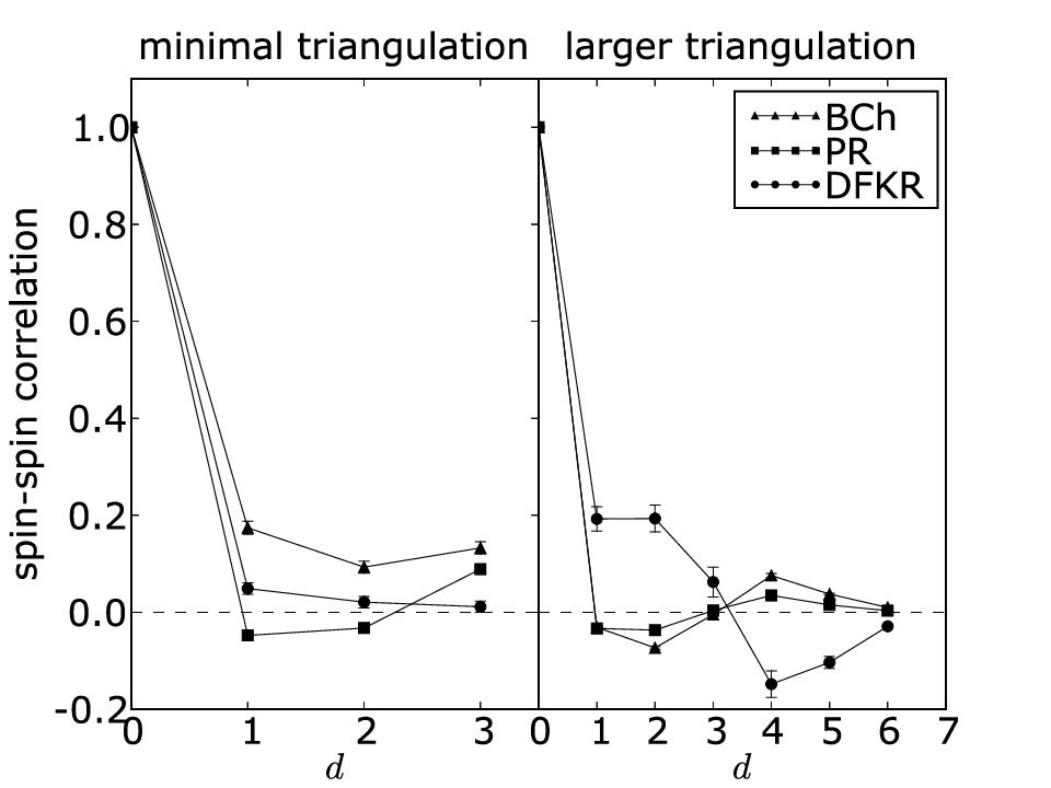
A small triangulation limits the maximum distance between faces. For example, the minimal triangulation has maximum distance $d=3$. Larger triangulations of the $4$-sphere were obtained by refining the minimal one by applying Pachner moves randomly and uniformly over the whole triangulation. We restricted the Pachner moves to those that did not decrease the number of simplices.

The largest triangulation we have used has maximum distance $d=6$. Its correlations for different models are shown in Figure 6 along with those from the minimal triangulation. Correlation functions for different values of ROU parameter $r$ (including the $q=1$ case) and other triangulations are qualitatively similar.

Notice the small negative dip for small values of $d$ for the Perez-Rovelli and Baez-Christensen models. As discussed in previous sections, the partition functions of these models are dominated by spin foams with isolated bubbles. The correlation data is consistent with this hypothesis. The values of the spins assigned to faces of the bubble will be strongly correlated, while the values of the spins on two faces, one of which lies on the bubble and the other does not, should be strongly anti-correlated. Since a given face usually has fewer nearest neighbors that lie on the same bubble than that do not, on average, the short distance correlation is expected to be negative. At slightly larger distances, the correlation function turns positive again. This indicates that on a larger triangulations, spin foams with several isolated bubbles contribute strongly to the partition function. Although, with so few data points, it is difficult to extrapolate the behavior of the correlation function to larger triangulations and distances, its features are qualitatively similar to that of a condensed fluid, where the density-density correlation function exhibits oscillations on the scale of the molecular dimensions.

Note that the behavior of the DFKR correlation function is significantly different from the other two. This is also consistent with the already observed fact that its partition function has strong contributions from other than single or isolated bubble spin foams.