Analysis of random Boolean networks using the average sensitivity

In 1969 Stuart Kauffman started to study random Boolean networks as simple models of genetic regulatory networks [1]. Random Boolean networks that consists of a set of Boolean gates that are capable of storing a single Boolean value. At discrete time steps these gates store a new value according to an initially chosen random Boolean function, which receives its inputs from random chosen gates. We will give a more formal definition later. Kauffman made numerical studies of random networks, where the functions are chosen from the set of all Boolean functions with $K$ arguments (the so called $NK$-Networks). He recognised that if $K\leq 2$, the random networks exhibit a remarkable form of ordered behaviour: The limit cycles are small, the number of ineffective gates, which are gates that can be perturbed without changing the asymptotic behaviour, and the number of freezing gates that stop changing their state is large. In contrast if $K\geq 3$, the networks do not exhibit this kind of ordered behaviour (see [1, 2]). The first analytical proof for this phase transition was given by Derrida and Pomeau (see [3]) by studying the evolution of the Hamming distance of random chosen initial states by means of so called annealed approximation. The first proof for the number of freezing and ineffective gates was given by James Lynch (see [4], although slightly weaker results appeared earlier [5, 6]). Depending on a parameter $\lambda$, that depends on the probabilities of the Boolean functions, he showed that if $\lambda\leq 1$ almost all gates are ineffective and freezing, otherwise not. Although his analysis is very general, until now it was only applied to networks with connectivity $2$ and non-uniform probabilities for the Boolean function: if the probability of choosing a constant function is larger or equal the probability of choosing a non-constant non-canalizing function (namely the XOR- or the inverted XOR-function), $\lambda$ is less or equal to one. But it turns out that in some cases $\lambda$ is equal to the expectation of the average sensitivity. Therefore we will first study the average sensitivity in Section 3. Afterwards it will be shown in Section 4 how to use the results from the previous section to apply Lynch’s analysis to classical $NK$-Networks and biased random Boolean networks ¹¹ 1 a definition will be given later. But first we will give some basic definition used throughout the paper in Section 2.

In the following $\mathbb{F}_{2}=\left\{0,1\right\}$ denotes the Galois field of two elements, where addition, denoted by $\oplus$, is defined modulo 2. The set of vectors of length $K$ over $\mathbb{F}_{2}$ will be denoted by $\mathbb{F}_{2}^{K}$. If ${\mathbf{x}}$ is a vector from $\mathbb{F}_{2}^{K}$, its $i$th component will be denoted by ${\mathrm{x}_{i}}$. With ${\mathbf{u}}^{(i)}\in\mathbb{F}_{2}^{K}$ we will denote the unit vector which has all components zero except component $i$ which is one. The Hamming weight of ${\mathbf{x}}\in\mathbb{F}_{2}^{K}$ is defined as

and the Hamming distance of ${\mathbf{x}},{\mathbf{y}}\in\mathbb{F}_{2}^{K}$ as

A Boolean function is a mapping $f:\mathbb{F}_{2}^{K}\rightarrow\mathbb{F}_{2}$. A function $f$ may be represented by its truth table ${\mathbf{t}}_{f}$, that is, a vector in $\mathbb{F}_{2}^{2^{K}}$, where each component of the truth table gives the value of $f$ for one of the $2^{K}$ possible arguments. To fix an order on the components of the truth table, suppose that its $i$th component equals the value of the corresponding function, given the binary representation (to $K$ bits) of $i$ as an argument.

In this section we will focus on the average sensitivity. The average sensitivity is a known complexity measure for Boolean functions, see for example [7]²² 2 here it is called critical complexity. It was already used to study Boolean and random Boolean networks for example in [8, 9].

Now consider the random variable $F_{K}:\Omega\rightarrow{\cal F_{K}}$, where ${\cal F_{K}}$ denotes the set a all $2^{2^{K}}$ Boolean function with $K$ arguments. The probability measure is given by $P(F_{K}=f)=\frac{1}{2^{2^{K}}}$. The expected value of the average sensitivity of this random variable is denoted by $\mathbb{E}_{F_{K}}(s_{f})$, and is given by

The expected value was already derived in [10], and is given by:

We will now concentrate on biased Boolean functions. The bias of a Boolean function $f:\mathbb{F}_{2}^{K}\rightarrow\mathbb{F}_{2}$ is defined as the number of $1$ in the functions truth table divided by ${2^{K}}$. To define the bias of a random Boolean function two definitions are possible. First we can assumes that the truth tables of the Boolean functions are produced by independent Bernoulli trials with probability $p$ for a one (This should be called mean bias, used for example in [3, 8] ). Therefore consider the random variable $F_{K,p}$. The probability of choosing a function $f$ is given by

For $p=1/2$ this is equivalent to the definition of $F_{K}$.

As a second possibility, we can only choose functions which have bias $p$ whereas to all other functions we assign probability 0 (we will call this fixed bias). Therefore consider the random variables $F^{\text{fixed}}_{K,p}:\Omega\rightarrow{\cal F_{K}}$. Denote the truth table of a function $f$ by ${\mathbf{t}}_{f}$. Further denote the set of all Boolean functions $f$ with $K$ arguments and $\wH({\mathbf{t}}_{f})=p2^{K}$ with ${\cal F}_{K,p}$. The probability for a certain function chosen according $F^{\text{fixed}}_{K,p}$ is given by

Both definitions ensure that the expectation to get a one is equal to $p$ if the input of a function is chosen at random (with respect to uniform distribution). But it will turn out that these two different methods of creating biased Boolean functions, have a major impact on the average sensitivity.

The expectation of the average sensitivity of $F_{K,p}$ was derived in [8]:

For the random variable $F^{\text{fixed}}_{K,p}$ we will now proof the following theorem:

It should be noted, that the Theorems 1 and 2 can be proved using in a similar way. Also worth noting is the fact, that if the functions are chosen according $F_{K},F^{\text{fixed}}_{K,p}$ or $F_{K,p}$ the expectation of the sensitivity of a fixed vector ${\mathbf{w}}$ (namely the expectation of $s_{f}({\mathbf{w}})$) is independent of ${\mathbf{w}}$ (see Equation (1),(2), (3) and (4)). Hence the following lemma holds

Before proceeding to the next section, it should be noted, that using the same arguments as in the proof of Theorem 3, we can also prove the expectation of average sensitivity of order $l$ , defined as

In this case, instead of summing up all unit vectors in Equation (1), we sum up all vectors of Hamming weight $l$. As the equations (2) and (4) hold for all ${\mathbf{w}}\in\mathbb{F}_{2}^{K}$ we conclude that

and by similar arguments

respectively

As already mentioned James Lynch gave a very general analysis of randomly constructed Boolean networks (see [4]). Before stating his results we give a formal definition for Boolean networks A Boolean network B is a 4-tuple $(V,E,\tilde{F},{\mathbf{x}})$ where $V=\{1,...,N\}$ is a set of natural numbers, $E$ is a set of labeled edges on $V$, $\tilde{F}=\{f_{1},...,f_{N}\}$ is a ordered set of Boolean functions such that for each $v\in V$ the number of arguments of $f_{v}$ is the in-degree of $v$ in $E$, these edges are labeled with $1,...,\text{\emph{in-degree}}(v)$, and ${\mathbf{x}}=({\mathrm{x}_{1}},\dots{\mathrm{x}_{n}})\in\mathbb{F}_{2}^{N}$. Suppose that a vertex $i$ has $K_{i}$ in-edges from vertices $v_{i,1},\dots,v_{i,K_{i}}$. For ${\mathbf{y}}\in\mathbb{F}_{2}^{N}$ we define

The state of B at time 0 is called the initial state ${\mathbf{x}}$, so we define ${\mathbf{B}}^{0}({\mathbf{x}})={\mathbf{x}}$. For time $t\geq 1$ the state is inductively defined as ${\mathbf{B}}^{t}({\mathbf{x}})={\mathbf{B}}({\mathbf{B}}^{t-1}({\mathbf{x}}))$. Hence we can in interpret $V$ as set of gates, $E$ and $\tilde{F}$ describes their functional dependence and ${\mathbf{x}}$ is the networks initial state.

Assume some ordering $f_{1},f_{2},...$ on the set of all Boolean functions $\cal F$, where each function $f_{i}$ depends on $K_{i}$ arguments. Further a random variable $F:\Omega\rightarrow{\cal F}$ with probabilities $p_{i}=P(F=f_{i})$ such that $\sum_{i=i}^{\infty}p_{i}=1$ and $\sum_{i=1}^{\infty}p_{i}K_{i}^{2}<\infty$. Now a random Boolean network consisting of $N$ gates is constructed as follows: For each gate a Boolean function is chosen independently, where the probability of choosing $f_{i}$ is given by $p_{i}$. Suppose a function $f$ was chosen that has $K$ arguments, these arguments are chosen at random from all $\binom{N}{K}$ equally likely possibilities. At last an initial state is chosen at random from the set on all equally likely states. If the Boolean functions are chosen according to our previously defined random variable $F_{K}$ we will call this networks $NK$-Networks with connectivity $K$. If the functions are chosen according to $F^{\text{fixed}}_{K,p}$ or $F_{K,p}$ we will call this networks biased random Boolean networks with connectivity $K$ and fixed bias $p$ respectively mean bias $p$.

Let us now state Lynch’s results. His analysis depends on a parameter $\mathbb{R}\ni\lambda\geq 0$ depending only on the functions and their probabilities. We will define $\lambda$ later in Definition 3. First we have to state Lynch’s definition of freezing and ineffective gates:

Now we will state the main result.

The above theorem shows that if $\lambda\leq 1$ almost all gates are freezing and ineffective and otherwise not. The next corollary gives us more information what happens if $\lambda>1$:

Now we will state the definition of $\lambda$ for Boolean networks:

Obviously $\gamma(f,{\mathbf{w}})$ is identical to $s_{f}({\mathbf{w}})$ which will be used instead in the further discussion. The constant $a$ is the probability that a random gate is one (at infinite time) given that all gates at time $0$ have probability $0.5$ of being one. (see [4, Definiton 2]). Assume that we choose the functions according a random variable $F$ which should be either $F_{K}$, $F^{\text{fixed}}_{K,p}$ or $F_{K,p}$. The functions are chosen out the set ${\cal F}_{K}$, we denote a function’s probability with $p_{f}$. It follows that

${\mathbb{E}}(s_{F}({\mathbf{w}}))$ denotes the expectation of the sensitivity for a fixed ${\mathbf{w}}$, Equation (7) follows from Lemma 1. Therefore, together with Theorem 1 and Theorem 3 we proved the following:

As a special case of the above theorem we get (or by using Theorem 1)

The results about $NK$-Networks are consistent with experimental results. In fact if $K\leq 2$ almost all networks almost all gates are freezing and almost all gates are ineffective and otherwise not (see [2]).

Obviously, the border between the ordered and disordered phase is given by $\lambda=1$. The resulting phase diagram for biased random Boolean networks, where the functions are chosen according to $F^{\text{fixed}}_{K,p}$ and $F_{K,p}$ is shown in Figure 1. It it interesting to note that if the functions are chosen with fixed bias, then also Boolean networks with connectivity $K=2$ can become unstable. This conclusion can be drawn from Lynch’s original result already. As mentioned in the introduction, he showed for $K=2$, that $\lambda>1$ if the probability of choosing a non-constant non-canalizing function, namely the XOR or the inverted XOR function, is larger than the probability of choosing a constant function. For example if the bias is $0.5$, the probability of choosing a constant function is zero, whereas both XOR and inverted XOR function have probability greater zero, hence $\lambda>1$.

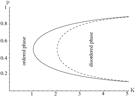
It is interesting to compare our results with previous results obtained first by Derrida and Pomeau using the so called annealed approximation (see [3]). In their annealed model the functions and connections are chosen at random at each time step. Considering two instances of the same annealed network starting in two randomly chosen initial states ${\mathbf{s}}_{1}(0),{\mathbf{s}}_{2}(0)$ they show that

where $c=1$ if

and $c\leq 1$ otherwise. It is remarkable that the two models behave similar, but it is unclear whether this holds in general.

We would like to thank our colleges Georg Schmidt and Stephan Stiglmayr for proofreading and Uwe Schoening for useful hints.

References

- [1] S. Kauffman, Metabolic stability and epigenesis in randomly constructed nets, Journal of Theoretical Biology 22 (1969) 437–467.
- [2] S. Kauffman, The large scale structure and dynamics of genetic control circuits: an ensemble approach, Journal of Theoretical Biology 44 (1974) 167–190.
- [3] B. Derrida, Y. Pomeau, Random networks of automata - a simple annealed approximation, Europhysics Letters 2 (1986) 45–49.
- [4] J. F. Lynch, Dynamics of random boolean networks, in: Conference on Mathematical Biology and Dynamical Systems, University of Texas at Tyler, 2005.
- [5] J. F. Lynch, On the threshold of chaos in random boolean cellular automata, Random Structures and Algorithms (1995) 236–260.
- [6] J. F. Lynch, Critical points for random boolean networks, Physica D: Nonlinear Phenomena 172 (1-4) (2002) 49–64.
- [7] I. Wegener, The Complexity of Boolean Functions, Wiley-Teubner Series in Computer Science, John Wiley, B.G. Teubner, 1987.
- [8] I. Shmulevich, S. A. Kauffman, Activities and sensitivities in boolean network models, Physical Review Letters 93 (4).
- [9] S. Kauffman, C. Peterson, B. Samuelsson, C. Troeln, Genetic networks with canalyzing boolean rules are always stable, Proceedings of the Nationial Academy of Science 101 (49).
- [10] A. Bernasconi, Mathematical techniques for the analysis of boolean functions, Ph.D. thesis, Dipartimento di Informatica, Universita di Pisa (March 1998).